4
$\begingroup$

I simulated a discrete sample of a variable whose autocorrelation function (ACF) should theoretically be composed of a sum of exponential-like functions.

My goal is to represent it in the frequency domain because that is how it is done experimentally. This is theoretically achieved by calculating the Fourier-Laplace transform of the time derivative of the ACF with changed sign.

The difficulty is that the process occurs in a complex system and does not contain $N$ isolated and easily identifiable exponentials, but a scattered mixture from which hopefully you can detect $M<N$ main contributions. EDIT: If it contained those few easily identifiable exponentials, I could identify them and move analytically into the frequency domain. Since this is not the case, I have tried to do it numerically, but I get too much noise in the results.


What I tried

I have tried several methods but I have no experience in signal processing and I do not know which one is the most reliable. The most significant of these are:

  1. Direct method: Just compute the ACF and perform the FFT. I get a lot of noise in the ACF and even more after transform it. I've noticed some seasonality.

  2. Smoothing/Averaging: I made a windowed version of the Savitzky-Golay filter and applied it to the ACF, this improved the results but not sufficiently. Dividing the ACF in blocks and averaging it gave significant improvements.

  3. Welch’s method: This returned the spectral density. I applied the IFFT to get the ACF which looks much nicer than previous approaches. I keep the first half (because the returned ACF looks like a periodic function), and then applied the FFT to its derivative.

The latter results looks way better but with issues: 3.1) The imaginary part of the frequency representation does not tends to zero at zero frequency (it is smaller that its peak, but not close to zero). 3.2) I have not found which window would be appropriate for the FFT. The ones I have seen have small values at the extremes, and the ACF has valuable information and higher accuracy near $t=0$.

  1. Parametric methods: Assume that the process follows the autoregressive model (AR), estimate its order through AICc test, get the corresponding coefficients of the AR and found 'analytically' the power spectra. Perform the IFFT and then the FFT. The final result looks pretty nice but some assumptions where made.

Questions
  1. Which window should I use considering that the time representation is an exponential like function with more precise and meaningful information at small $t$?

  2. It is reasonably to compute the power spectra, apply the IFFT to get the ACF and then the FFT to the derivative of it first half? If so, why the imaginary part is not zero at zero frequency?

  3. Should I use the Welch's method or the parametric one?


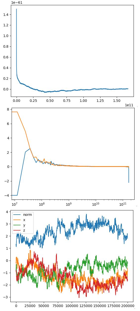
Three plots

Botton: Components and norm of the vector function simulated (400 000 samples).

Top: 1D-Autocorrelation function computed using the IFFT of the spectral density (obtained via Welch's method).

Middle: FFT of the derivative of the padded above ACF.

$\endgroup$
12
  • $\begingroup$ Could you supply some examplary diagrams to help us get a better understanding of what we're dealing with here? $\endgroup$
    – Max
    Commented Jan 6, 2022 at 6:59
  • $\begingroup$ @Max Thank you for reply! Please excuse the delay. I added three images, I hope they help. $\endgroup$ Commented Jan 12, 2022 at 18:29
  • $\begingroup$ Your problem specification seems to suggest methods that analyse the eigenstructure of the autocovariance matrix. This will give you a decomposition into exponential functions. $\endgroup$
    – Jazzmaniac
    Commented Feb 1, 2022 at 14:00
  • $\begingroup$ @Jazzmaniac Thank you. I do not know how to arrive to a decomposition into exponential functions from the eigen vectors of the autocovariance. However, I cannot see the advantage over the 4th mentioned approach. Also, I need just a few exponentials prior move to freqs domain, otherwise I could just project onto a linear combination of exponential functions. Could you elaborate a little more on this subject? $\endgroup$ Commented Feb 1, 2022 at 17:14
  • $\begingroup$ I actually don't understand the question. Are you having issues creating the data samples? Are you having issues with analysis of the data generated in the simulation? The question is really unclear to me. $\endgroup$
    – Royi
    Commented Feb 7, 2022 at 6:54

1 Answer 1

1
+100
$\begingroup$

I suspect in looking at the plots that the underlying process is non-stationary. The PSD as the FT of the ACF only exists for stationary processes. What you can potentially do for non-stationary processes is run the signal through a high-pass filter which converts many non-stationary processes to a stationary process (and removes the lowest frequency components which may be out of the area of interest). The lower the cut-off, the lower in frequency you can go for evaluating the higher spectral components, but only up to the point where stationarity can be assumed. Many processes suffer from "1/f noise" and "drift of the mean" which appears as an increase in the noise power spectral density as we get lower and lower in frequency. This ultimately violates our assumption of stationarity. In statistics this is also done with a differencing filter, which as a high pass filter can be used to eliminate wander and drift of the mean as well as filter out increasing low frequency noise components (but for spectral analysis a simple high-pass would be better suited due to the "comb" response of a difference filter).

The Allan Variance is an excellent metric to determine the interval in which stationarity can be assumed. The Allan Variance is a 2-sample variance which utilizes differencing to establish a consistent variance metric. The variance of the difference of two averaged blocks of the signal in time averaged over $\tau$ seconds, with each block seperated by $\tau$ seconds. For a stationary process, the Allan Variance will continue to decrease as $\tau$ increases. Once the Allan Variance ceases to go down is the time interval over which stationarity can no longer be assumed. That said you can use this information to compute a PSD over a direct interval of the waveform up to $\tau$ seconds, or if a longer interval is needed then a high-pass filter with a cut-off of $1/\tau$ can potentially be applied to extend this time further. It is for this reason specifically that the Allan Variance is a popular tool for the evaluation of oscillators when considering their long term accuracy performance. Phase Noise is a good short term assessment but can not be measured beyond time intervals in which stationarity can not be assumed, and the phase noise for all oscillators is non-stationary in the long term (but will be stationary over short time intervals). This is why you typically do not see phase noise power spectral densities with frequency offsets below 0.1 Hz to 10 Hz depending on the frequency of the source and it's long term drift performance. That said, the Allan Variance is a useful measurement tool for all similar processes that are not stationary in a longer term of interest.

I detail the Allan Variance (and associated Allan Deviation or "ADEV") in these other posts:

Allan Variance vs Autocorrelation - Advantages

How to interpret Allan Deviation plot for gyroscope?

Is it possible to add some kind of noise to a non stationary (having unit root) signals to make them stationary?

What determines the accuracy of the phase result in a DFT bin?

That said, I recommend that the OP review the "ADEV" for the waveform (the Python library "allantools" is excellent) and determine the longest $\tau$ interval in which stationarity can be assumed (this is the point where the ADEV plot bottoms out), and then use that time interval to compute the PSD. The PSD can be computed in multiple blocks over $\tau$ with the final result averaged to emulate "Video BW". The time interval used for $\tau$ would represent "Resolution BW". I explain those terms in the context of spectral analysis further here.

$\endgroup$
8
  • $\begingroup$ +1 Thank you for your answer, it is very useful to me. I'll follow your suggestion. The sample is about ten times longer than needed by the resolution requirements.I'd tried to split the sample in many parts (using not clear criteria) and compute de ACF of each one and then average them before going to freq domain. The result looked much better. You suggest compute and average PSDs. Am I doing the conversion to freq domain (real/imaginary parts) in a right way?(applying IFFT to the PSD get the ACF and then the FFT..).Also, could you provide any link to a recommendable moving difference filter? $\endgroup$ Commented Feb 7, 2022 at 13:20
  • $\begingroup$ I wouldn't do the moving difference filter if the block length doing it block by block is acceptable and use Welch's method with that maximum block length where stationarity applies. If the spectrum is generally noise without significant (many 10's of dB variation in power level, then windowing would not be necessary). $\endgroup$ Commented Feb 7, 2022 at 13:29
  • $\begingroup$ Thank you! I understood that (except I didn't know about the tip in the parenthesis). I still do not know if the block length doing it block by block is acceptable. I am just reading the allantools docs and I really have a lot of samples of different system to analyse and compare. I asked for a link because I am afraid that I will need one of these "moving difference filters" in the future and will not know what to do then (I googled the term and find something like X(n) = [x(n)-x(n-1)]/2, but I think that it is not what are you are referring to). $\endgroup$ Commented Feb 7, 2022 at 13:50
  • $\begingroup$ The differencing filter results in a "comb" response so for spectral analysis specifically of a non-stationary process a standard high-pass filter would be better suited. I'll update my answer to reflect that. $\endgroup$ Commented Feb 7, 2022 at 17:05
  • 1
    $\begingroup$ Yes that is a good plan. You are only using ADEV to confirm that the block length you want to use for Welch’s is suitable. The block length (and window chosen) sets your resolution bandwidth. The subsequent averaging of blacks then smooths the noise as a result of giving you a tighter “video bandwidth”. You find these same knobs on a spectrum analyzer (test equipment) $\endgroup$ Commented Feb 8, 2022 at 12:36

Your Answer

By clicking “Post Your Answer”, you agree to our terms of service and acknowledge you have read our privacy policy.

Not the answer you're looking for? Browse other questions tagged or ask your own question.