Unwanted periodicity in data

Question

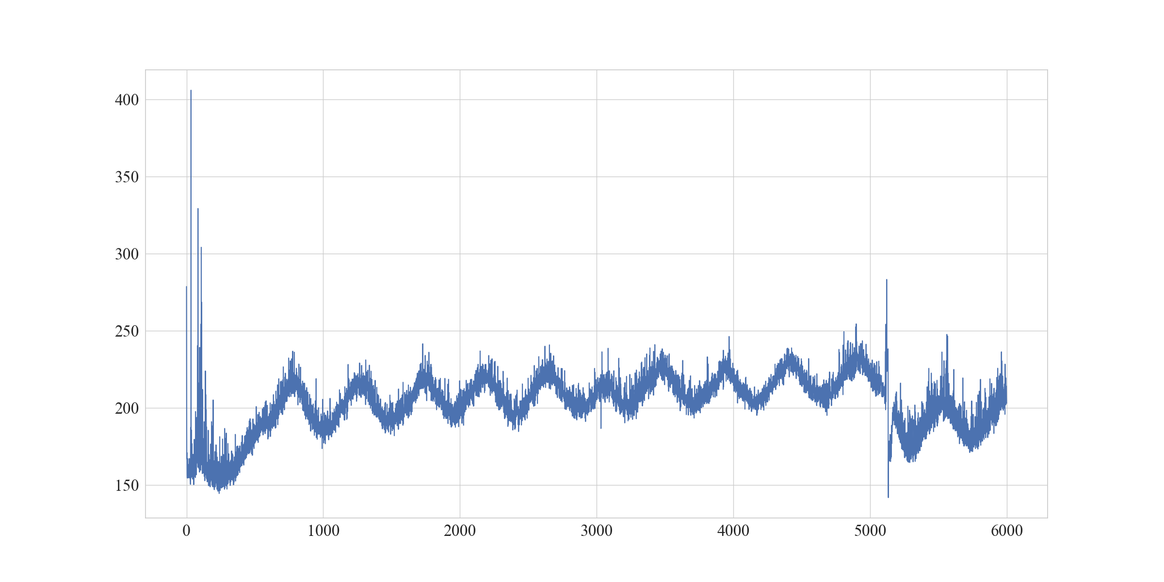
my signal consists of data points that represent the (vibration signal) energy measured during process cycles of a machine. Due to the hydraulic power units emptying and filling again, some periodicity is introduced into the yielding signal of energy measurements.

I am searching for a way to remove this periodicity from the data, since this effect persists over the course of all data points, however I am interested in changes in the signal that do not stem from this physical effect.

Sadly, my DSP skills are very limited, so I am hoping that someone could help me. I work with Python.

Please find attached I) an image of a data sample and II) a sample from the data.

I

II https://pastebin.com/rgxhhmcH // Password zzxWgpFxYb

Addition: Sadly I don't have the opportunity to get the signal from the hydraulic units. The original signal was sampled with 1MHz. From these signals I calculated the energy for each process cycle. Every 1.2s one process cycle was carried out. However, there are breaks between process cycles, e. g. at ~5100 (see image).

Answer 1

Some time-frequency analysis with the synchrosqueezed CWT, where I guess fs=10000 but this doesn't matter except for axis labels and physical interpretation.

1. Take SSQ_CWT of original, tune wavelet for sparsity

Tune parameters until we get the most energy concentration in the fewest number of points. The signal appears to have detailed low frequency behavior, which makes CWT the suitable tool of choice as opposed to STFT.

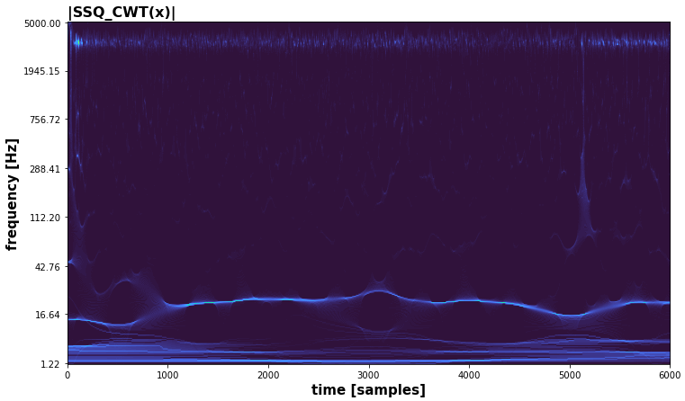
The clear curve we see confirms this, and it's what we want to eliminate according to OP.

2. Filter the undesired

Applying SSQ inversion, which is a highly non-linear inversion that can't be achieved with FFT-based methods, we obtain

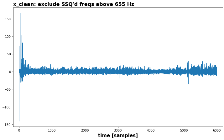
Granted, due to the simple inversion specification in this case (exclude freqs entirely), other methods may achieve similar results.

3. Take SSQ_CWT again to see what we've got, re-tune for sparsity

I also zoomed along freq. Need to change wavelet again due to the tightly-packed nature of higher frequencies in this signal (need better frequency resolution).

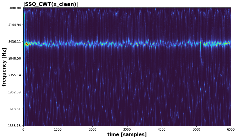
Zoom along time since it's hard to see:

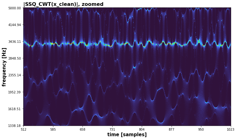
4. Filter the undesired, round 2

The non-intense regions appear noisy - they may not be noise, but they're complicated enough that some highly nonlinear methods will be required, possibly neural nets, to make sense of them. Given that this is just machinery and not brain EEG, it's likelier noise. Zoomed along time, plus amplitude envelope:

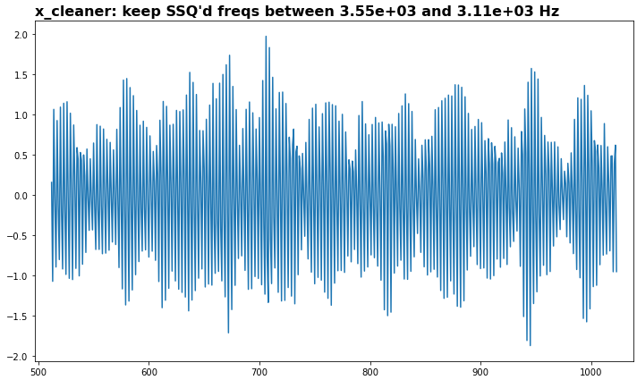
and in SSQ:

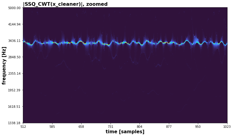
5. Inspect amplitude via Hilbert transform

Not entirely appropriate since the single component isn't quite clean - SSQ would do better but it's a lot of work, but we should get a good approximation:

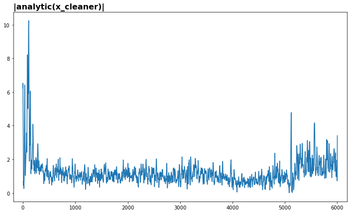
Now take its SSQ

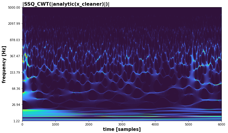
No strong pattern, looks like noise - makes sense as the measurement is mediated by a bunch of physical processes and nothing to push the measurement intensity a specific way.

Verdict

The signal of interest is most likely an AM-FM waveform, the FM being sine-like and AM being noisy. It's considerably different from a pure sine, but depending on application, a pure sine wouldn't be a terrible approximation. A higher sampling rate would aid with further insights, as the FM bandwidth is tightly packed.

Messy code

import numpy as np
from scipy.signal import hilbert
from ssqueezepy import ssq_cwt
from ssqueezepy.visuals import plot, imshow

FS = 10000
# x = # load data

ikw = dict(abs=1, xlabel="time [samples]", ylabel="frequency [Hz]")

Tx, _, ssq_freqs, *_ = ssq_cwt(x, ('gmw', {'gamma': 1, 'beta': 10}), fs=FS)

imshow(Tx, yticks=ssq_freqs, **ikw, title="|SSQ_CWT(x)|")

x_clean = Tx[:100].sum(axis=0).real
plot(x_clean, xlabel="time [samples]",  show=1,
     title="x_clean: exclude SSQ'd freqs above %.3g Hz" % ssq_freqs[99])

#%%
Tx, _, ssq_freqs, *_ = ssq_cwt(x_clean, ('gmw', {'gamma': 3, 'beta': 30}), 
                               fs=FS, nv=256)
imshow(Tx[:500], yticks=ssq_freqs[:500], **ikw, title="|SSQ_CWT(x_clean)|",
       norm=(0, np.abs(Tx).max()/10))

imshow(Tx[:500, 512:1024], yticks=ssq_freqs[:500], **ikw, 
       xticks=np.arange(512, 1024),
       title="|SSQ_CWT(x_clean)|, zoomed", norm=(0, np.abs(Tx).max()/10))
x_cleaner = Tx[130:180].sum(axis=0).real
#%%

plot(np.arange(512, 1024), x_cleaner[512:1024], 
     title="x_cleaner: keep SSQ'd freqs between %.3g and %.3g Hz" % (
         ssq_freqs[130], ssq_freqs[180]), show=1)

#%%
Tx, _, ssq_freqs, *_ = ssq_cwt(x_cleaner, ('gmw', {'gamma': 3, 'beta': 30}), fs=FS,
                               nv=256)

imshow(Tx[:500, 512:1024], yticks=ssq_freqs[:500], **ikw, 
       xticks=np.arange(512, 1024),
       title="|SSQ_CWT(x_cleaner)|, zoomed", norm=(0, np.abs(Tx).max()/10))


xca = np.abs(hilbert(x_cleaner))
plot(xca, title="|analytic(x_cleaner)|", show=1)
#%%
Tx, _, ssq_freqs, *_ = ssq_cwt(xca, ('gmw', {'gamma': 3, 'beta': 10}), fs=FS,
                               nv=256)
imshow(Tx, **ikw, norm=(0, np.abs(Tx).max()/10), yticks=ssq_freqs,
       title="|SSQ_CWT(|analytic(x_cleaner)|)|")