Understanding FFTs for simple Circular Function (sin/cos)

Question

Background : This is my first question in this forum, and although I read several threads on this side and googled a lot I could not find the answer to my question (maybe it is too basic)?

For anyone reading this thread with a similar question: The code is now adapted in a way that the answer is partly given in this question. For the explanations look in the answers below.

I found this one, but it only covered my answer partly. If you have good literature that covers this topic, I'm grateful if you can share it.

So, let's assume I have a very basic signal in the time domain. For example, $5\sin(3\cdot2\pi x-2)$ with Amplitude as $5$, Frequency as $3$ and Shift of $2$.

import matplotlib.pyplot as plt
import numpy as np
npts  = 100
tmax  = 10
dt = tmax / npts
fs = 1 / dt
t     = np.linspace(0, tmax-dt, npts)
y     = 5 * np.sin(3 * 2*np.pi * t - 2)
N = y.size

freq = np.fft.fftshift(np.fft.fftfreq(N)*fs)
yfft = np.fft.fft(y)
yfft = np.where(abs(yfft) < 1.0e-10, 0, yfft)
magn = np.fft.fftshift(np.abs(yfft*dt)/(N*dt))
phase = np.fft.fftshift(np.angle(yfft))
psd = np.fft.fftshift(np.abs(yfft*dt)**2/(N*dt))
yfft = np.fft.fftshift(np.fft.fft(y))

How do I get the frequency $3$ and the shift of $2$ to show? Is that even possible?

fig, ax = plt.subplots(3, 2)
fig.tight_layout()
ax[0,0].plot(t, y)
ax[0,0].set_title('Time-Domain')
ax[0,1].plot(freq, yfft)
ax[0,1].set_title('Frequency-Domain')
ax[1,0].plot(freq, magn)
ax[1,0].set_title('Magnitude')
ax[1,1].plot(freq, phase)
ax[1,1].set_title('Phase')
ax[2,0].plot(freq, psd)
ax[2,0].set_title('PSD')

Answer 1

Creating the Frequency Vector

The arrangement of the output of fft() depends on whether you use an odd or even number of points for your fft. I think this post nicely summarises how the frequencies are arranged. Have a look at it.

• Since you are using an even number of points, the Nyquist frequency, $F_N = F_s/2$, is present in the output of your fft, and is the maximum value in your frequency vector. Your sampling frequency is $N/T=100/10=10\;\textrm{Hz}$, and so your maximum detectable frequency in the vector will be $F_N=5\;\textrm{Hz}$.
• Secondly, no matter whether you use even or odd points, the DC value is always the first entry in the fft output.
• The frequency resolution $df = F_s/N$ is the separation between fft output bins in frequency space. For you, this will be $0.1\;\textrm{Hz}$.
• Finally, it is also most common to display the frequency spectrum in a symmetric, centered way, with the DC frequency in the middle - the function fftshift does this for you.

Accounting for all this, your frequency vector corresponding to your fft output (after you have applied fftshift() to centre it) will be $$ f = [-F_N : df : (F_N-df)] $$ There is some discussion about fftshift in this thread if you are interested. Notice that after fftshift() the component corresponding to the Nyquist, $F_N$, is placed at the beginning of the vector, and so is considered a negative frequency from the point of view of fftshift() - there is no Nyquist at the end of the vector in the positive frequencies (then in contrast, for symmetry, the DC component is viewed as a positive frequency).

Plotting the Spectrum with Correct Scaling

Personally, I prefer to deal with these things in terms of the power of a wave (rate of change of energy) instead of the amplitude of a component in a fft bin. This just helps me to keep track of the units, and to keep things physical. The following code calculates the power spectral density, $S_{xx}$, for your signal using a simple periodogram estimate (I assume your signal is in volts - may or may not be true - but could be anything: temperature, stock prices, etc). Sorry, but my code is in Matlab, not Python, but hopefully you can follow the steps without problem.

N = 100;   % Number of samples
T = 10;    % Record window duration
dt = T/N;  % Sampling period
Fs = 1/dt; % Sampling frequency

t = 0:dt:(T-dt); % Time vector for sampling

% generate samples at the specified times
x = 5*sin(2*pi*3*t - 2); % units: [V]

df = Fs/N; % frequency resolution (bin width in frequency space)

% generate frequency vector for 2-sided spectrum (NOTE, this arrangement
% only works for even number of points - otherwise, use f = -(Fs/2-df/2):df:(Fs/2-df/2))
f = -(Fs/2):df:(Fs/2-df);

% Calculate Fourier transform (approximating CFT), and shift DC term to centre
X = fftshift(fft(x))*dt; % units: [V sec]

X((abs(X)<1e-10)) = 0; % kill values below threshold, so phase is well-behaved

% Calculate power spectral density using periodogram estimation
Sxx = (X.*conj(X))/(N*dt); % units: [V^2 / Hz]

figure; stem(f,Sxx)      % Plot power spectral density
figure; stem(f,angle(X)) % Plot phase

The variable $X$ in the code is a discrete approximation of the continuous Fourier transform integral, which is why it is multiplied by the sampling period $dt$ (the approximation is a Riemann sum). Then the periodogram can be calculated from this - again, in a discrete version of its continuous counterpart, which is explained very nicely I think in this answer. Note, Matlab also has a built-in function periodogram(), which does the calculation as well.

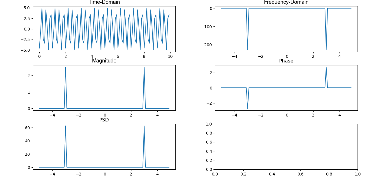
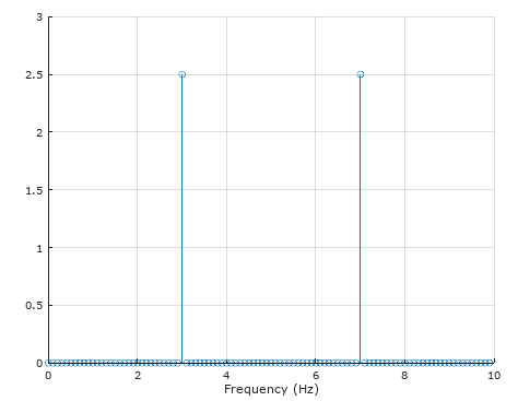
You can see that there are peaks correctly at $\pm 3\;\textrm{Hz}$, matching exactly your input signal (remember the sin wave is actually a sum of complex exponentials).

-- Note that in signal processing, the "energy" is defined as [signal squared multipled by time], and so therefore power is given as [energy per time], which is then [signal squared]. This is why you see "power" in my answer given in units of $[V^2]$. To find the physical power in [Watts] you would simply need to scale by the resistance of whatever the load is you are driving. This is usually set to 1 in signal analysis --

Verifying Parseval's Theorem

You can also verify the scaling of the fft output by checking that the power and energy in both the time domain and frequency domain are equal, as they should be according to Parseval's Theorem. Remember that if you integrate the power spectral density over all frequencies, you should obtain the total power that was present in the input signal. For example, using

Energy_timedomain = sum(x.*conj(x))*dt  = 125  [V^2 sec]
Power_timedomain = Energy_timedomain/T  = 12.5 [V^2]
Energy_freqdomain = sum(X.*conj(X))*df  = 125  [V^2 sec]
Power_freqdomain = sum(Sxx)*df          = 12.5 [V^2]

Note that if you take a longer time window duration $T$ for your input signal then the "energy" will increase (because there is more of it), but the average power will stay the same (because that is the rate of change of energy).

Recovering the Amplitude

The value of each peak in the power spectral density plot is $62.5\; [\textrm{V}^2 / \textrm{Hz}]$. To convert this to power, we need to multiply by the bin width (essentially integrating the power spectral density over that bin). In your case, the bin width is $df=F_s/N = 10\;\textrm{Hz}/100 = 0.1\;\textrm{Hz}$. Therefore, the total power in the input signal at that frequency is $$ P = 2 \times 62.5\;[V^2/\textrm{Hz}] \times 0.1\;[\textrm{Hz}] = 12.5\;[V^2] $$ where the factor of $2$ is because there are 2 peaks - half of the power in the negative part of the spectrum and half in the positive part. Note that if your input signal is real, then the output spectrum will always be symmetric, and you will often see the negative frequencies (which don't contain any extra information) discarded. If you choose to throw away the negative frequencies then you should multiply the power in the unique positive frequencies that are left by 2 to compensate (but don't multiply the DC or the Nyquist by 2, because there are only one of each of those in the fft output - they don't have negative counterparts).

We know that for sinusoids the power and amplitude $A$ are related by $P = A^2/2$ (again, just setting any load resistance to $1$). Therefore, rearranging this, your amplitude of the 3 Hz wave is

$$A = \sqrt{2\times 12.5} = 5\;[V]$$

Recovering Phase

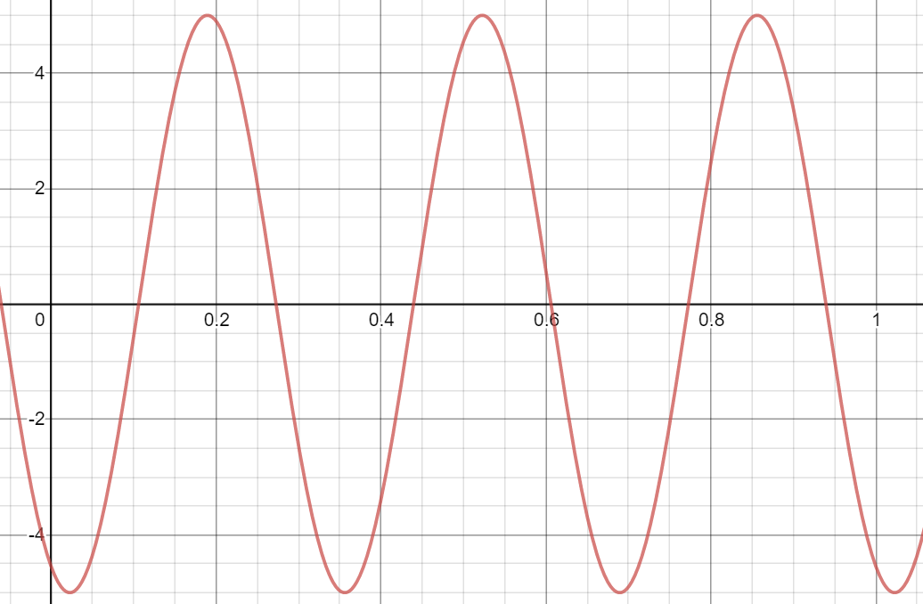
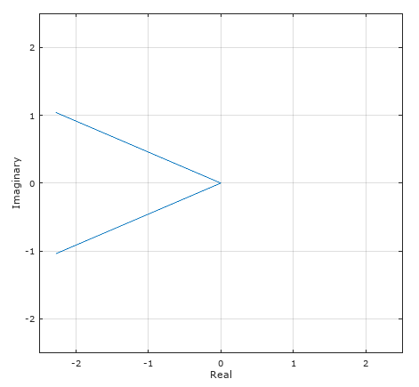
As Hilmar said, the phase of $-2$ can be recovered by taking the phase value at $3\;\textrm{Hz}$, which is 2.712, and adding $\pi/2$ then subtracting $2\pi$. The $\pi/2$ is because your input signal is a sine wave, which essentially includes a phase shift already because $$ \sin(2\pi f_0 t + \phi) = \cos(2\pi f_0 t + (\phi - \pi/2)) = \cos(2\pi f_0 t + \phi_{\textrm{fft}}) $$ so you need to add $\pi/2$ to the phase returned by the fft() to get your input phase $$\phi = \phi_{\textrm{fft}} + \pi/2 = 2.712 + \pi/2 = 4.283.$$ The final $2\pi$ subtraction is because after doing this you are left with something greater than $\pi$, and so you just need to unwrap the phase to bring it back into the range $[-\pi ... +\pi]$.

A FINAL NOTE OF CAUTION It all works nicely in this case because all of your signal energy falls exactly in a single fft bin, due to the combination of the sampling rate, number of points, time window, and your input frequency wave (see here). Things are more difficult if you have any windowing or zero-padding applied to your input signal before you pass it to fft(). There are some enlightening answers here and here, when you get that far.

Answer 2

Know that each bin in the FFT is the value for the exponential $e^{j\omega t}$, not sine or cosine.

So for the OP's case $5sin(2\pi 3 x-2)$ in terms of exponentials (see Euler's identity) this is:

$$\frac{5}{2j}e^{j(6\pi x -2)} - \frac{5}{2j}e^{-j(6\pi x -2)}$$

Each is a DFT bin with that magnitude and phase given by the exponentials above, as long as the DFT is normalized by $1/N$. (the $1/j$ is just an additional phase shift of $e^{-j\pi/2}$, so for example the first bin will have a magnitude of $2.5$ and phase of $-2-\pi/2$).

Further the frequency axis in the DFT has an index of $k$ which goes from $0$ to $N-1$ for $N$ samples in the DFT which corresponds to the frequency axis going from $0$ to $(N-1)/N$ Hz, circularly rotated such that the upper part of the spectrum is equally the negative frequencies. This means with a sampling rate of $10$ Hz and $100$ samples, the $-3$ Hz frequency given above is equivalently $+7$ Hz:

$e^{-j(2\pi fx -\phi)}$ when sampled is $e^{(-j2\pi f n/f_s - \phi)}$

So the value above $\frac{5}{2j}e^{-j(6\pi x -2)}$ when sampled is $\frac{5}{2j} e^{-j(2\pi 3 n/10 -2)}$

This is equivalently $\frac{5}{2j}e^{-j(2\pi (10-3)n/10 -2)} = \frac{5}{2j}e^{-j(2\pi 7 n/10 -2)} $

So bottom line, the two bins corresponding to 3 Hz and 7 Hz will have the magnitude and phase given by the Euler's expansion of the sine wave given, when the DFT is properly scaled by $1/N$.

---

Showing this for the OP's example:

For your case it appears you have $N= 100$ with a sampling rate $f_s = 10$, so to ensure an integer number of cycles (MATLAB code below):

N = 100
fs = 10
n= 0:N-1;
f = 3;
y = 5*sin(2*pi*f*n/fs-2);

If you use the normalized DFT, which scales the answer by $1/N$ you get the following plot for the magnitude where we can clearly see the 2.5 coefficient as derived above, and the two tones (due to the cyclical property of the DFT the upper spectrum shown past 5 Hz represents the negative frequency axis: 5 Hz to 10 Hz is the same as -5 Hz to 0 Hz). Here I translated the bin number k to frequency using n/fs:

We can graphically see the phase of these two bins get this from the phase of those FFT bins as demonstrated below through a complex (real-imaginary) plot of the fft. We see each of the two bins as phasors with a magnitude of 2.5 and phase of $\pm 2.71$ radians, which is the same as $\pm 2\pi-2.71 = 3.57$ radians, or the expected $\pm(-2-\pi/2) = \pm 3.57$ radians:

Answer 3

A few points to consider.

This all gets a lot easier if you create a sine wave that has an integer number of periods in your time window. You can do this by building your time vector as

t = np.linspace(0, tmax*(1-1/npts), npts) 

If you do this you can approach this as follows:

1. You are using a time window of length of 10s sampled with 100 taps, which gives you a time resolution of 0.1s or a sampling rate of 10Hz.
2. The result of the FFT has 100 frequency bins with a bin spacing of 0.1Hz. You will find the FFT value corresponding to your 3 Hz sine wave in bin 30 = $3Hz/0.1Hz$ AND bin 70 = $(10Hz-3Hz)/0.1Hz$ . Bin 30 represent the positive frequency component, bin 70 the negative frequencies.
3. The amplitude in each bin will be FFTSize*Amplitude/2 = 250.
4. The phase of at the positive bin will be 2.7124. In order to get your original phase of -2 you need to add $\pi/2$ to compensate for the difference of sine and cosine and subtract $2\pi$ to unwrap the phase.

If your sine wave does NOT have integer number of periods, things get a whole lot more complicated and I wouldn't go there until you have fully understood the integer case.