1
$\begingroup$

I am using MATLAB for this question so hopefully you can help me out.

I am trying to compute the Wigner-Ville distribution (WVD) of a sinusoidal signal defined as \begin{equation} x(t) = e^{-i\omega_0 t} e^{i\phi(t)}, \end{equation} where $\omega_0$ is the central frequency (rad/s) and $\phi(t)$ is a Brownian phase noise function, defined as a random walk $\phi(t) = \sqrt{\Delta\Omega}W(t)$ and $W(t)$ is a Wiener process $W(t)\sim \sqrt{|t|} N(0,1)$. The parameter $\Delta\Omega$ represents the linewidth of my laser. The idea is that I can compute the auto-correlation function of $x(t)$ \begin{equation} r_x(t+\tau/2,t-\tau/2) = E\left[x(t+\tau/2)x^*(t-\tau/2)\right] = e^{-i\omega_0 \tau} e^{-\Delta\Omega |\tau|/2 }, \end{equation} where $E[\cdot]$ is the expectation operator or ensemble average. Once I compute this, I can then compute the average Wigner-Ville Distribution using \begin{equation} E[W(t,\omega)] = \int_{-\infty}^{\infty} r_x(t+\tau/2,t-\tau/2)e^{i\omega \tau}\ d\tau, \end{equation} Or essentially as the "Fourier transform" of the function $r_x$. This gives me the analytic formula \begin{equation} E[W(t,\omega)] = 2\frac{\Delta\Omega/2}{(\Delta\Omega/2)^2 + (\omega-\omega_0)^2}. \end{equation}

I can then compute the power spectral density (PSD) of $x(t)$ by integrating $E[W(t,\omega)]$ over $t$.

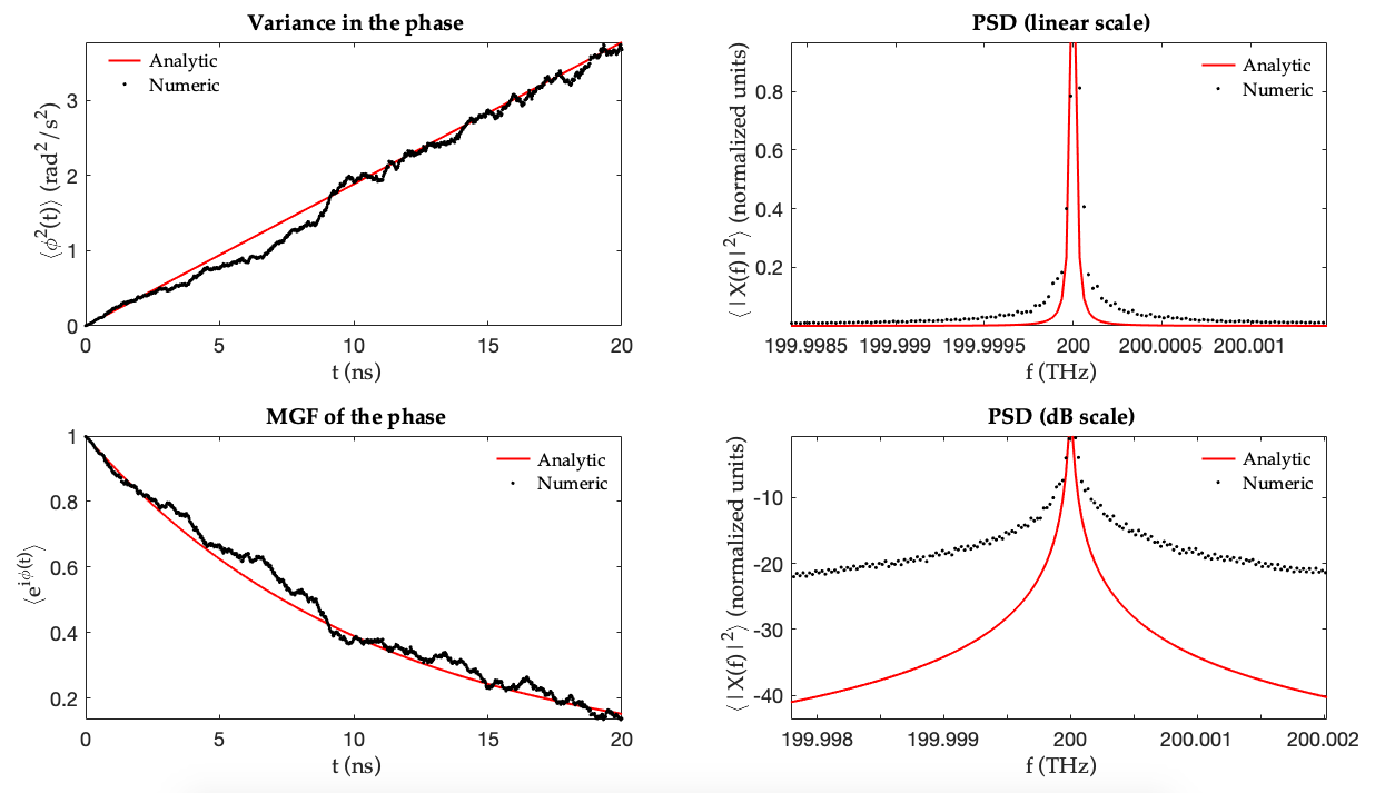
The problem now comes in when I try to replicate this result numerically, that is simulating $N$ random walks for $\phi(t)$, and creating a matrix $X$ which contains the signal on a time domain $t\in [0,T]$ for each of those random walks. I haven't been able to find any MATLAB functions that can compute the autocorrelation function $r_x$ for me, so instead I am trying to use the built-in function wvd() (Wigner-Ville distribution) directly on each of my $x$ simulations contained in the matrix $X$. The problem is that the result I get from the wvd() function has a different line-width in frequency space than the analytic (in fact the line-width of my function should be exactly $\Delta\Omega$, or simply $\Delta\nu = \Delta\Omega/2\pi$ when plotted on $f$ (Hz)), but that is not the case here (see plot below):

enter image description here

Does anyone know why this happens? Here is my MATLAB code:


%% --- INPUTS --- %%
% User-defined parameters
T = 20e-9;    % Time duraction of signal (s)
f0 = 200e12;  % Laser center frequency (Hz)
A = 1;        % Laser amplitude
FWHM = T/5;   % Full-Width at Half Maximum of Gaussian pulse
Nt = 1001;    % Sample points in time
Nf = Nt;      % Sample points in frequency
N_MC = 20;  % Monte Carlo Simulations
dNu = 30e6;   % Laser linewidth (Hz)

% Calculated parameters
w0 = 2*pi*f0;
dOm = 2*pi*dNu;
t = linspace(0,T,Nt);
dt = t(2)-t(1);
a = 4*log(2)/FWHM^2;
t0 = T/3;
df = 1/dt/Nf;
% f = f0 + df.*linspace(-Nf/2,Nf/2,Nf); % shift array to center f
% w = 2*pi*f;

% Signal
phi = @(t) sqrt(dOm)*cumsum(sqrt(dt)*randn(size(t))); % phase noise
x = @(t) exp(-1i*w0*t).*exp(1i*phi(t));

%% --- Analytic --- %%
% Signal properties
r_x = @(tau) A*exp(-1i*w0*tau).*exp(-dOm/2*abs(tau));
PSD_analytic = @(f) A*dOm./((dOm/2)^2 + 4*pi^2*(f-f0).^2);

% Phase properties
phi_var_analytic = @(t,dOm) dOm*abs(t);
phi_mgf_analytic = @(t,dOm) exp(-1/2*dOm*abs(t));

%% --- Numeric --- %%
% Phase properties
Tmatrix = columnVector(t).*ones(Nt,N_MC);
phi0 = phi(Tmatrix);
phi_var = mean( phi0.^2, 2) - mean(phi0,2).^2;
phi_mgf = mean( exp(1i*phi0), 2);

% Signal properties
x_samples = x(Tmatrix);
[f,Spectrum,PSD,comp_time] = WVS(t,x_samples,f0);
disp(['Computation time = ' num2str(comp_time/60) ' min']);

%% --- Plots --- %%
close all;
FS = '\fontname{Palatino} ';
fontS = 18;
colors = {'red','black'};
LW = 2;
factor0 = 50;
f00 = f0/1e12;
fmin0 = min(f)/1e12;
fmax0 = max(f)/1e12;
dfmax = (fmax0-fmin0)/2;
fmin = f00 - dfmax/factor0;
fmax = f00 + dfmax/factor0;

% ---> Phase Plots
figure('units','normalized','outerposition',[0 0 1 1]);
set(gcf,'color','w');

subplot(221);
plot(t*1e9,phi_var_analytic(t,dOm),'color',colors{1},'LineWidth',LW);
hold on;
plot(t*1e9,phi_var,'marker','.','color',colors{2},...
    'LineStyle','none','LineWidth',LW+1);
hold off; 
legend boxoff; legend([FS 'Analytic'], [FS 'Numeric']);
axis tight;
xlabel([FS 't (ns)']);
ylabel([FS '\langle' '\phi^2(t)\rangle (rad^2/s^2)']);
title([FS 'Variance in the phase']);
set(gca,'FontSize',fontS);

subplot(223);
plot(t*1e9,phi_mgf_analytic(t,dOm),'color',colors{1},'LineWidth',LW);
hold on;
plot(t*1e9,phi_mgf,'marker','.','color',colors{2},...
    'LineStyle','none','LineWidth',LW+1); hold off;
legend boxoff; legend([FS 'Analytic'], [FS 'Numeric']);
axis tight;
xlabel([FS 't (ns)']);
ylabel([FS '\langle' 'e^{i\phi(t)}\rangle']);
title([FS 'MGF of the phase']);
set(gca,'FontSize',fontS);

% ---> Spectral Plots (Normalized)
subplot(222);
plot(f/1e12,PSD_analytic(f)./max(PSD_analytic(f)),'color',colors{1},...
    'LineWidth',LW); hold on;
plot(f/1e12,PSD./max(PSD),'marker','.','color',colors{2},...
    'LineStyle','none','LineWidth',LW+1); hold off;
legend boxoff; legend([FS 'Analytic'], [FS 'Numeric']);
axis tight;
xlabel([FS 'f (THz)']);
ylabel([FS '\langle' '|X(f)|^2' '\rangle (normalized units)']);
title([FS 'PSD (linear scale)']);
set(gca,'FontSize',fontS);

subplot(224);
plot(f/1e12,10*log10(PSD_analytic(f)./max(PSD_analytic(f))),'color',...
    colors{1},'LineWidth',LW); hold on;
plot(f/1e12,10*log10(PSD./max(PSD)),'marker','.','color',colors{2},...
    'LineStyle','none','LineWidth',LW+1); hold off;
legend boxoff; legend([FS 'Analytic'], [FS 'Numeric']);
axis tight;
xlabel([FS 'f (THz)']);
ylabel([FS '\langle' '|X(f)|^2' '\rangle (normalized units)']);
title([FS 'PSD (dB scale)']);
set(gca,'FontSize',fontS);

%% --- Functions --- %%
function [freq,Spectrum,PSD,comp_time] = WVS(t_array,x_array,f0)
% Ensembled Averaged Wigner-Ville Distribution
% x_array: each column is a single ensemble of the random signal x(t)
N = length(t_array);
dt = abs(t_array(2)-t_array(1));
fs = 1/dt;
[~,N_MC] = size(x_array);
W = 0;
tic;
for n = 1:N_MC % Do ensemble averaging over multiple Monte Carlo samples
    [W0,f,~] = wvd(ifftshift(x_array(:,n)),fs);
    Nf = length(f);
    df = 1/dt/Nf;
    W = W + dt*W0;
    if rem(n,10)==0
        disp(n);
    end
end
freq = f0 + f - max(f)/2;
Spectrum = abs(fftshift(W/N_MC));
PSD = dt*trapz(Spectrum,2);
comp_time = toc;
end

function output = columnVector(input_vector)
[sx,sy] = size(input_vector);
if sx < sy
    output = input_vector.';
else
    output = input_vector;
end
end

PS: I know that my function $x(t)$ in this case is stationary (since $r_x$ depends only on $\tau=t-t'$ and not on two separate times $(t,t')$; and so I could calculate the PSD using the Wiener-Khinchin theorem, but I want to use the WVD instead so that my code can be generalized for non-stationary functions $x(t)$ (e.g. such as Gaussian pulses)

EDIT: I have changed my definition of phi(t) in the code so that it now is computed as a random walk with \begin{equation} \phi(t+\Delta t) = \phi(t) + \sqrt{\Delta\Omega}\sqrt{\Delta t}N(0,1), \end{equation} but this still does not solve the problem of the numerical PSD being a lot wider than the analytic PSD, and I can't figure out why

$\endgroup$
1
  • $\begingroup$ see Update on the tail asymptote $\endgroup$
    – V.V.T
    Commented May 8, 2021 at 11:10

1 Answer 1

1
$\begingroup$

Your formula for $\displaystyle W(t)$ does not represent a Wiener process.

By definition, the Wiener process ${\displaystyle W}$ has Gaussian increments: ${\displaystyle W_{t+u}-W_{t}}$ is normally distributed with mean ${\displaystyle 0}$ and variance ${\displaystyle u}$, ${\displaystyle W_{t+u}-W_{t}\sim {\mathcal {N}}(0,u)}$. Just because $\displaystyle W_t^2 − t$ is a martingale, does not result in your formula $\displaystyle W(t)\sim \sqrt{|t|} N(0,1)$.

You can easily see it, comparing two plots:

  • fill in an array $GN[1:N]$ with a realization of Gaussian process.
  • draw a plot for $sqrt(k)·GN[k]$
  • construct an array of partial sums, $W[k] = \sum_{i=1}^{i=k}GN[k]$, which is a realization of the Wiener process by definition
  • draw a plot for $W[k]$.

The jumps in the sequence $sqrt(k)·GN[k]$ increase with $k$ ($k$ represents discrete time); the jumps in the partial sums $W[k]$ vary around a Gaussian process variance and do not increase with $k$.

Notice also that there exists a representation of a Wiener process via i.i.d. Gaussian variable $ {\displaystyle ξ_{n}}$ in terms of a random Fourier series: $$ {\displaystyle W_{t}={\sqrt {2}}\sum _{n=1}^{\infty }ξ_{n}{\frac {\sin \left(\left(n-{\frac {1}{2}}\right)\pi t\right)}{\left(n-{\frac {1}{2}}\right)\pi }}} $$ on ${\displaystyle [0,1]}$. Comparing it to your formula for $W(t)$ is not a trivial task, but it indicates that you cannot just multiply the Gaussian noise realization with the time square root and have the Wiener process realization.

UPDATE on distribution tails

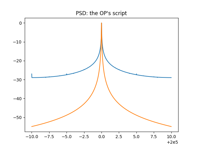
Numerical experiments with your script show that the tail asymptote might be on the order of $f^{-1}$. It is the behavior that one would expect in the system with the Brownian noise process: the prominent $1/f$ noise. On the other hand, the analytical formula that gives the expectation $E\left[W(t,ω)\right]$ of the Wiener process in the form of a Lorentz profile with a $\Delta \Omega$ parameter, may be wrong, seemingly disregarding the Wiener process at all. You can easily see it by comparing the pure Lorentz profile with the parameters of the Brownian noise process.

What's more, your script produces the numeric $1/f$ profile even without any noise. To prove it, I removed the phase noise from the signal generator. The noiseless signal is x = @(t) exp(-1i*w0*t). The PSD asymptote for this signal is $f^{-2}$, but your script still gives "a spectrum which is a lot wider than it should be, compared to the analytic result". The script is in Python, but you can translate it easily and nearly literally to MATLAB:

import numpy as np
import matplotlib.pyplot as plt
from scipy import signal
from scipy import fft, ifft
import tftb 

# --- INPUTS --- 
# User-defined parameters
T = 20    # Time duraction of signal (ns)
f0 = 200e3  # Laser center frequency (GHz)
Nt = 1000    # Sample points in time
dNu = 0.030   # Laser linewidth (GHz)

# Calculated parameters
w0 = 2*np.pi*f0
dOm = 2*np.pi*dNu
t = np.linspace(0,T-T/Nt,Nt)
dt = t[1]-t[0]

#--- Analytic --- 
#Signal properties
def PSD_analytic(f):
    return dOm/((dOm/2)**2 + 4*np.pi**2*(f-f0)**2)

#----Numeric ---
wvd = tftb.processing.WignerVilleDistribution(np.exp(-1j*w0*t), timestamps=t)
W,freq,_ = wvd.run()
PSD = np.abs(np.trapz(fft.fftshift(W), axis=1))
PSD_OP = np.trapz(np.abs(fft.fftshift(W)), axis=1)

f = f0 + freq - max(freq)/2

#--- Plots --- 
plt.figure(3)
plt.title("PSD: the OP's script");
plt.plot(f,10*np.log10(PSD_OP/np.max(PSD_OP)))
plt.plot(f,10*np.log10(PSD_analytic(f)/np.max(PSD_analytic(f))))
plt.figure(4)
plt.title("PSD: use projection property");
plt.plot(f,10*np.log10(PSD/np.max(PSD)))
plt.plot(f,10*np.log10(PSD_analytic(f)/np.max(PSD_analytic(f))))
plt.show()

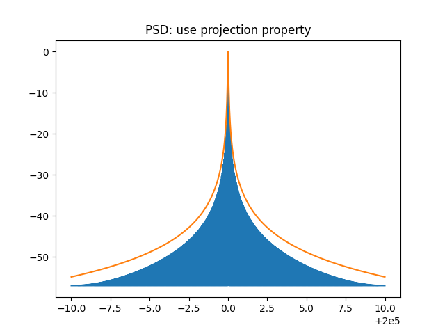
The array PSD_OP is produced according to your script recipe. Comparing the two expressions for PSD, your PSD_OP = np.trapz(np.abs(fft.fftshift(W)), axis=1) and corrected PSD = np.abs(np.trapz(fft.fftshift(W), axis=1)), one sees the reason why the tails of your distribution deviate from the Lorentzian's $f^{-2}$ law. The PSD can be obtained from the Wigner-Ville distribution using the Projection property $$ |X(f)|^2 = \int_{-\infty}^\infty W_x(t,f)\,dt $$ (PSD = np.abs(np.trapz(fft.fftshift(W), axis=1))

projection_property

while your script replaces it with $$ |X(f)|^2 = \int_{-\infty}^\infty |W_x(t,f)|\,dt $$ (PSD_OP = np.trapz(np.abs(fft.fftshift(W)), axis=1))

OP_script

The WVD(x(t)) envelope of the noiseless x(t) = exp(-1j*w0*t) signal is the sign-flipping sinc function; the asymptote of its frequency projection is an $f^{-2}$.

With the positive function abs(sinc()) integrated over time, the asymptote retains the $f^{-1}$ asymptote of abs(sinc(2πft)).

Providing the highest possible temporal-vs-frequency resolution among the other time-frequency analysis tools, the WVD function still has its caveats. Also, I do not discuss the physics behind your research, but please, decide for yourself, what laser pulse model you are using. Specifically, your script retains some vestiges of working with a Voigt profile (FWHM, a = 4*np.log(2)/(FWHM*FWHM), maybe of a Gaussian broadening), but x(t_array) = np.exp(1j*(phi(t_array)-w0*t_array)) might suggest the pulse train model. It is not quite clear what model of laser pulse you are simulating.

To answer your original question, I attach the Python script based on your MATLAB's with some corrections. The corrections only deal with the signal processing issues.

import numpy as np
import matplotlib.pyplot as plt
from scipy import signal
from scipy import fft, ifft
import tftb 

# --- INPUTS --- 
# User-defined parameters
T = 20    # Time duraction of signal (ns)
f0 = 200e3  # Laser center frequency (GHz)
A = 1        # Laser amplitude
FWHM = T/5   # Full-Width at Half Maximum of Gaussian pulse
Nt = 1000    # Sample points in time
Nf = Nt      # Sample points in frequency
N_MC = 100    # Monte Carlo Simulations
dNu = 0.030   # Laser linewidth (GHz)

# Calculated parameters
w0 = 2*np.pi*f0
dOm = 2*np.pi*dNu
t = np.linspace(0,T-T/Nt,Nt)
dt = t[1]-t[0]
a = 4*np.log(2)/(FWHM*FWHM)
t0 = T/3
df = 1/dt/Nf

# Signal
def phi(t):
    return np.cumsum(np.sqrt(dt*dOm)*np.random.randn(*np.shape(t)),axis=0) # phase noise TODO: axis=0?
def x(t):
    return np.exp(1j*(phi(t)-w0*t))

#--- Analytic --- 
#Signal properties
def r_x(tau):
    return A*np.exp(-1j*w0*tau)*np.exp(-dOm/2*abs(tau))
def PSD_analytic(f):
    return A*dOm/((dOm/2)**2 + 4*np.pi**2*(f-f0)**2)

#Phase properties, moment generating function
def phi_var_analytic(t,dOm):
    return dOm*np.abs(t)
def phi_mgf_analytic(t,dOm):
    return np.exp(-1/2*dOm*abs(t));

#--- Numeric --- 
#Phase properties
Tmatrix = t[:,np.newaxis]*np.ones((Nt,N_MC))
phi0 = phi(Tmatrix)
phi_var = np.mean( phi0**2, axis=1 ) - np.mean(phi0, axis=1)**2
phi_mgf = np.mean( np.exp(1j*phi0), axis=1 )

#Signal properties
x_samples = x(Tmatrix);

#--- Functions --- 
def WVS(t_array,x_array,f0):
    # Ensembled Averaged Wigner-Ville Distribution
    # # x_array: each column is a single ensemble of the random signal x(t)
    N = len(t_array);
    dt = abs(t_array[1]-t_array[0]);
    ts = np.arange(N) * dt 
    _,N_MC = np.shape(x_array)
    wvd = tftb.processing.WignerVilleDistribution(fft.ifftshift(x_array[:,0]), timestamps=ts)
    W,f,_ = wvd.run()
    # Do ensemble averaging over multiple Monte Carlo samples
    for n in range(1,N_MC-1):
        wvd = tftb.processing.WignerVilleDistribution(fft.ifftshift(x_array[:,n]), timestamps=ts)
        W0,f,_ = wvd.run()
        W = W + dt*W0
    freq = f0 + f - max(f)/2
    spectrum = fft.fftshift(W/N_MC)
    PSD = np.abs(np.trapz(spectrum, axis=1))
    return [freq,spectrum,PSD]

f,spectrum,PSD = WVS(t,x_samples,f0);

#--- Plots --- 
plt.figure(1)
plt.title("Variance in the phase");
plt.plot(t,phi_var)
plt.plot(t,phi_var_analytic(t,dOm))
plt.figure(2)
plt.title("MGF of the phase");
plt.plot(t,phi_mgf)
plt.plot(t,phi_mgf_analytic(t,dOm))
plt.figure(3)
plt.title("PSD (linear scale)");
plt.plot(f,PSD/np.max(PSD))
plt.plot(f,PSD_analytic(f)/np.max(PSD_analytic(f)))
plt.figure(4)
plt.title("PSD (dB scale)");
plt.plot(f,10*np.log10(PSD/np.max(PSD)))
plt.plot(f,10*np.log10(PSD_analytic(f)/np.max(PSD_analytic(f))))
plt.show()

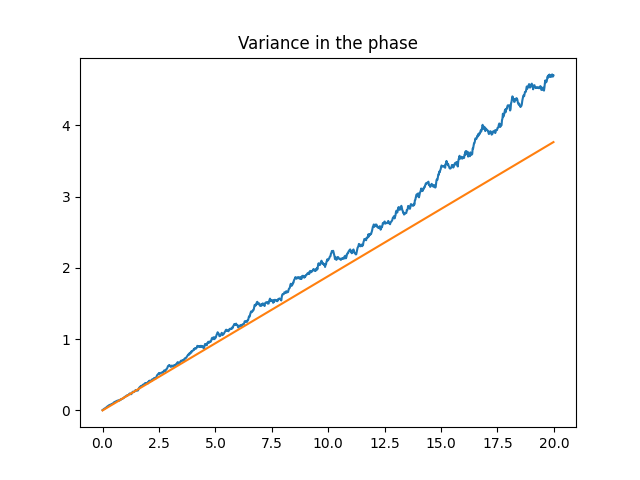
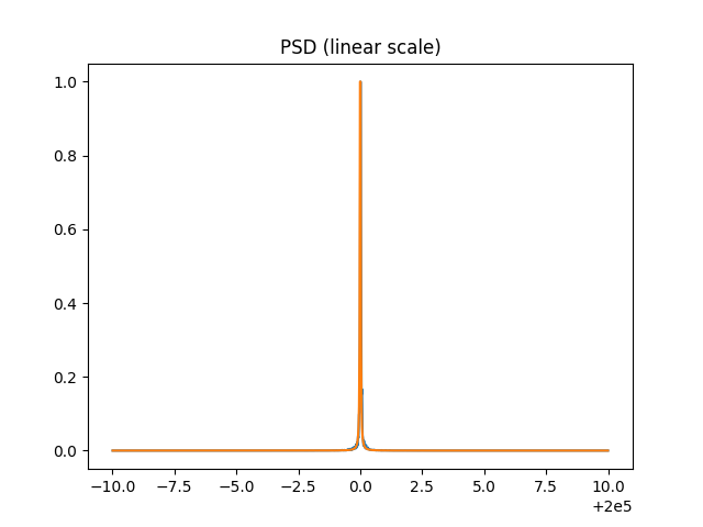
Figure_1

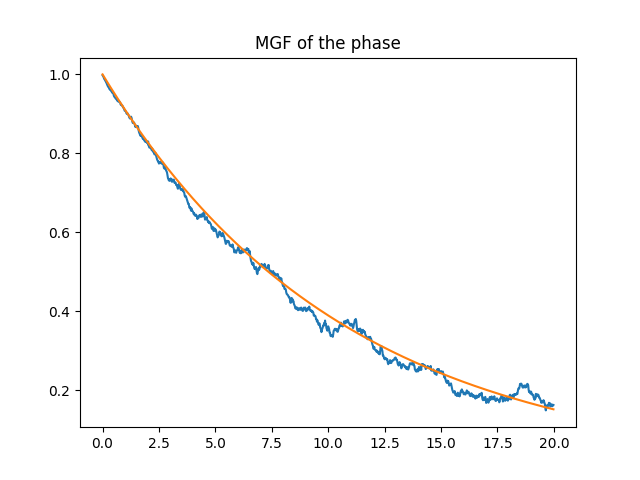
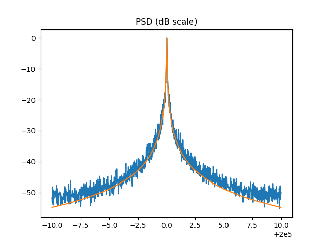
Figure_2

Figure_3

Figure_4

The PSD is much closer to the Lorentzian profile with these corrections, and the remaining discrepancy is due to "Wiener process" broadening from the signal processing point of view. Whether it has some physics in it is another question.

$\endgroup$
1
  • $\begingroup$ Yes this is correct, I had defined phi(t) wrong in my code. I have adjusted it so that it now is computed as a random walk via the equation: phi(t+dt) = phi(t) + sqrt(DeltaOmega)*sqrt(dt)*randn. However, that sill doesn't solve my problem. The main issue is that the frequency spectrum that results from using the Wigner-Ville Distribution function in matlab (wvd()) gives me a spectrum which is a lot wider than it should be, compared to the analytic result and I can't figure out if my implementation of wvd() is wrong $\endgroup$
    – OAN
    Commented Feb 13, 2021 at 2:32

Your Answer

By clicking “Post Your Answer”, you agree to our terms of service and acknowledge you have read our privacy policy.

Not the answer you're looking for? Browse other questions tagged or ask your own question.