Amplitude and Phase Recovery of a Signal Embedded in Linear Signal with Noise

Question

I have a noisy signal that has an ac component of fixed frequency but variable amplitude and phase. I'd like to recover the ac component.

The signal (blue trace) is mostly smooth, but has a few larger discontinuities.

The phase and amplitude of the ac component vary with time, this is how the signal looks like (green). Noise not shown:

The sampling rate is not commensurate with the ac period, this causes the aliasing seen in the picture. Unfortunately I cannot change this.

From this data, I need to recover amplitude and phase of the ac component, if possible also the harmonics.

My current approach is to multiply the data with a sine and cosine and then use a LPF to recover the quadrature components. I am not too happy with that approach, as the aliasing requires a very low cutoff frequency that smears out sharp transitions in the phase.

Also, I'd like to explore the solution space with some global constraints on amplitude and phase, e.g. sparsity and piece-wise continuity of the phase.

What is the right approach for phase and amplitude recovery? Can this be treated as a constraint convex optimization problem, or are there better solutions?

Update:

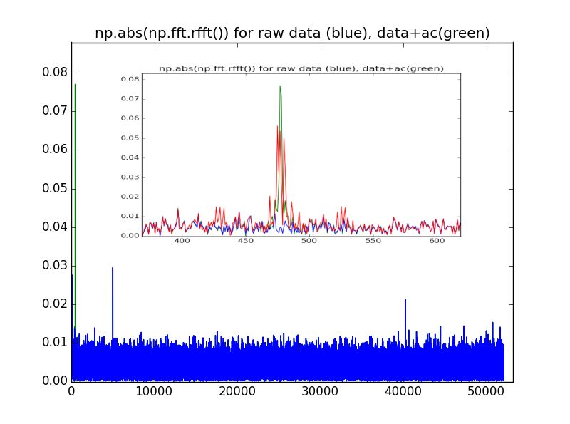
I have taken some real measurement data. I didn't have any data with the ac signal, so I have added an ac component numerically. The ac peak due to the signal is the highest green peak close to DC. The other two blue peaks are due to a digitizer artifact. The green curve is pretty much the same as the blue one in front elsewhere. This curve did not have any modulation on the ac signal, for a real signal, the peak would be about 2/3 that high and have some sidebands. This is shown in the inset image, the red curve is for the amplitude and phase modulated signal.

# simulated raw data for first plot
d=[0] * 50 + [1]*50 + list(np.linspace(0.5,1,50)) + list(np.exp(np.linspace(0,-1,30)))
# with additional small signal ac overimposed. Normally amplitude and phase would change as well
ds=d + 0.1*np.sin(100*np.linspace(0,6,180))
plt.plot(ds)

This is what I meant with global constraints: The data is very noisy, and it is not realistic to measure amplitude and phase without any averaging. On the other hand, I have some hypotheses about amplitude and phase, and would like to make use of them for filtering the data. For example, I know that there are sharp transitions in the phase, with areas of constant phase in-between. I don't want to average out the transitions. So ideally, I would like to recover the instantaneous amplitude and phase of the ac signal and then use a LASSO-like method to filter.

Answer 1

Assuming the problem is the signal being added to a piece wise linear signal I thought it would be good to eliminate it.

The problem is we're not given the samples index of each sample.
Hence we need to estimate this.

The idea to estimate this is as following:

1. Build a distance matrix for each pair of samples. The distance between 2 samples is the MSE of the linear estimator over the segment of samples.
   It means the 3 main diagonals of the distance matrix are zero.
   We also set that point which are far away have distance of infinity regardless of the MSE.
2. Cluster the data using this distance matrix.
   We can create affinity matrix / graph matrix and then look for the "sub graphs". Those are our segments.
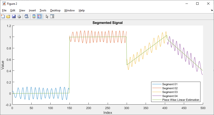
3. Once we have segments, per segment create the linear estimator.
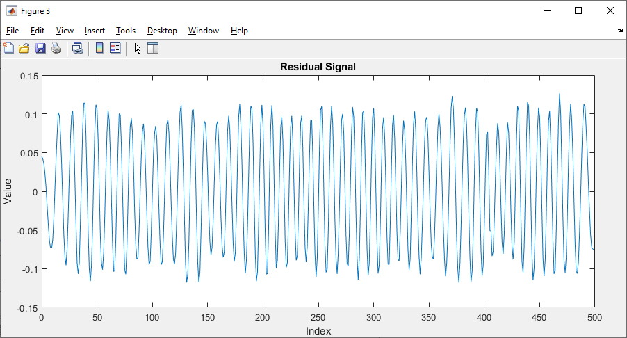
4. Calculate the residual per samples vs. its linear estimator.

Once you do this, you're left with harmonic signal which you may use all known methods to estimate its parameters (See ).

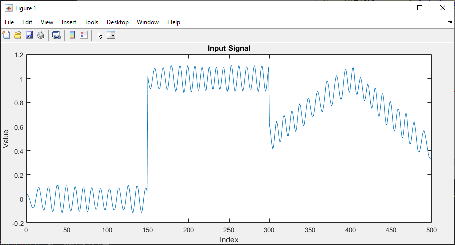
To show a proof of concept on a generated signal which looks similar to yours.

Remark: It would be great if you supplied your own signal as a CSV file or MAT file.