Benefit of Anti-Aliasing for Wideband Finite Time Duration Signals prior to Sampling

Question

Most literature about sampling explains the need for anti-alias filters in terms of periodic signals, preventing a periodic signal with frequency greater than half the sampling frequency from appearing as a mirrored low frequency signal.

However I acquire transient signals (not periodic) in my measurements, one-sided exponential pulses which have a very fast (high frequency) component followed by a slow decay (lower frequency). These are wideband signals. Quantities I care about are the timing of the fast edge, the integral of the pulse, and the rate of decay of the pulse. For timing measurements, a constant group delay is fine.

All of these measurements are taken using ADCs, for the equipment we use there is usually an anti-aliasing filter, 2nd order linear phase, with 3db attenuation at half the sampling frequency.

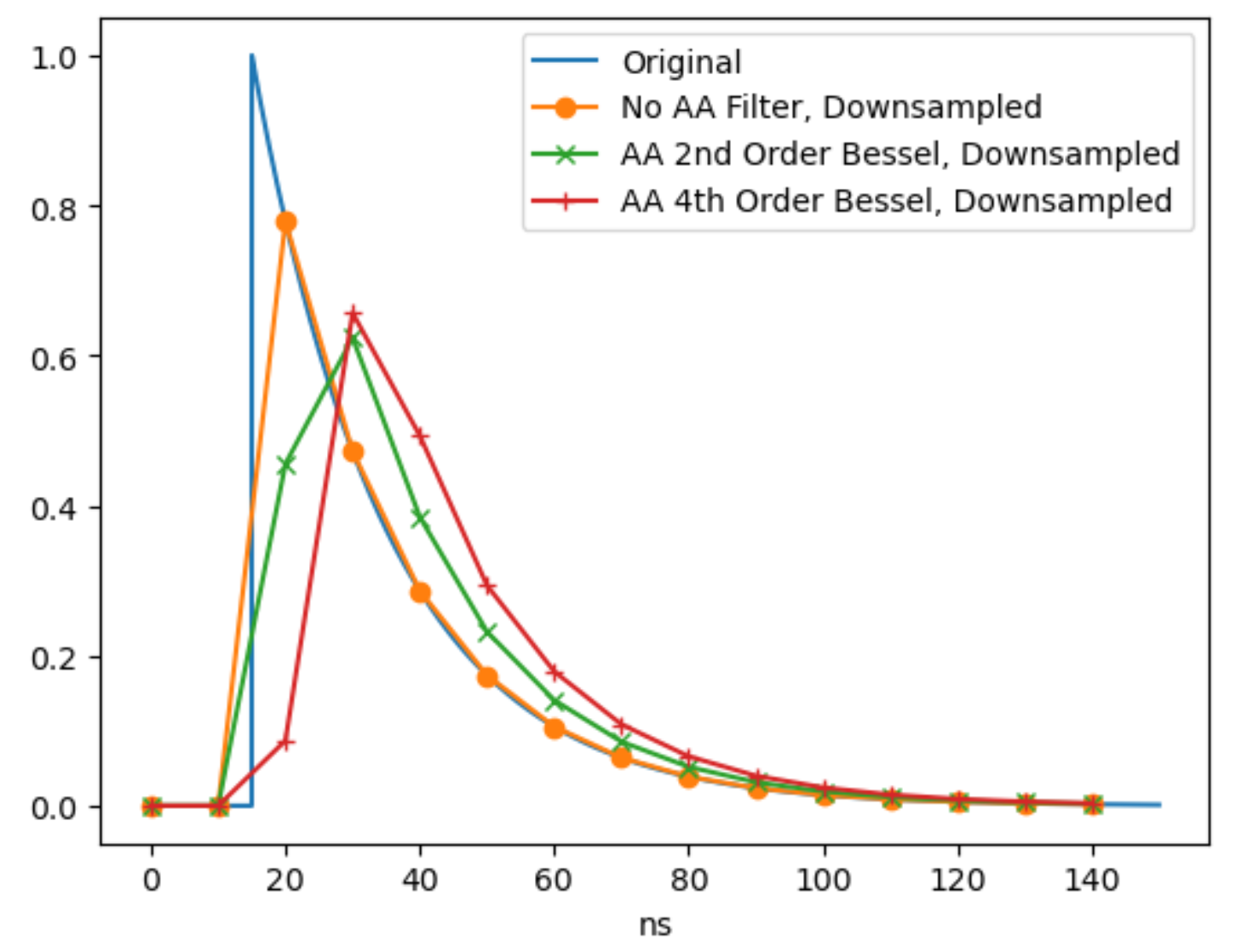
An exponential pulse, with simulated output after applying linear phase AA filters and downsampling is shown here

import numpy as np
from astropy import units as u
from astropy.visualization import quantity_support
quantity_support()
import scipy
import matplotlib.pyplot as plt

def t_range(time_length, n):
    return np.linspace(0 * time_length.unit, time_length, n+1)[:-1]

def freq_from_t(t, n=None, unit=u.MHz):
    if n is None:
        n = len(t)
        
    f = np.fft.rfftfreq(n, t[1]-t[0]).to(unit)

    return f

def apply_sample_rate(t, signal, sample_rate, filter_order=2):
    if filter_order is None:
        signal_filtered = np.copy(signal)
    else:
        f = freq_from_t(t)
        cutoff = sample_rate.to(u.MHz) / 2
        f_frac = cutoff / f[-1].to(u.MHz)
        sos = scipy.signal.bessel(filter_order, f_frac, output='sos')
        signal_filtered = scipy.signal.sosfilt(sos, signal)
    
    # now filter the signal
    samp_step_t = (1 / sample_rate).to(t[0].unit)
    t_sampled = np.arange(start=t[0].value, stop=t[-1].value, step=samp_step_t.value) * t[0].unit
        
    signal_filtered_sampled = np.interp(t_sampled, t, signal_filtered)

    return t_sampled, signal_filtered_sampled

t = t_range(150 * u.ns, 10000)
signal = np.exp(-(t-(15 * u.ns)) / (20 * u.ns))
signal[t < 15 * u.ns] = 0

sampling_freq = 100 * u.MHz

plt.plot(t, signal, label='Original')
plt.plot(*apply_sample_rate(t, signal, sampling_freq, filter_order=None), '-o', label='No AA Filter, Downsampled')
plt.plot(*apply_sample_rate(t, signal, sampling_freq, filter_order=2), '-x', label='AA 2nd Order Bessel, Downsampled')
plt.plot(*apply_sample_rate(t, signal, sampling_freq, filter_order=4), '-+', label='AA 4th Order Bessel, Downsampled')
plt.legend()

My question, is what benefit is an AA filter providing for these short pulses? Is an AA filter necessary at all? I can do my measurements on sampled waveform with no AA filter just fine. I am not considering noise yet, but trying to understand if an AA filter has any benefit in this ideal case.

Answer 1

I am going to appear to contradict something that Dan Boschen said* in his answer. I'm not really contradicting -- just putting a markedly different spin on it than he did.

You should use anti-aliasing filtering when, and to the extent that, using it gives you a better answer than not using it.

That's nebulous -- what do I mean?

If the amount of signal degradation that you get without using anti-aliasing is less than your system's desired accuracy, you don't need anti-aliasing. This can be the case when you have an impulsive signal and low additive noise.

"Light" (i.e., less than you might think based on a surface reading of the material) anti-aliasing filtering can be better than heavy brick-wall anti-aliasing filtering if the amount of signal degradation is as good as or better than the heavy anti-aliasing filtering, or no anti-aliasing filtering at all.

It sounds like your problem has the following properties:

• A pulse of known shape -- specifically, it's a decaying exponential of the form $u(t - t_0) A e^{-\frac{t - t_0}{\tau}}$.
• Little or no significant added noise.
• Unknown pulse amplitude ($A$).
• Unknown pulse timing ($t_0$).
• Unknown pulse time constant ($\tau$)

If these are all true, then without anti-alias filtering you can know $\tau$ with precision as good as your lack of noise. $t_0$ will be uncertain within a sampling interval, and $A$ will be uncertain to a factor of $e^{\frac{T_s}{\tau}}$, where $T_s$ is the sampling interval.

You can verify the above by noting that for zero noise and for $T_s (n-1) < t_0 \le T_s n$, any possible input signal in the family $$x(t) = u(t - t_0) A e^{-\frac{t - T_s n}{\tau}} e^{-\frac{T_s n - t_0}{\tau}}\tag 1$$ will all look identical.

If this is good enough -- stop, you've done your job, don't sweat any more.

If you do need to know $A$ and $t_0$ more accurately, then yes, an anti-aliasing filter will benefit you.

First, with an anti-aliasing filter that has a DC gain of unity (or a known DC gain that you can factor out), the area under the curve of any samples within an event will equal the area under the curve of the actual source signal.

Second, as long as the pulses are big enough and long enough compared to your filter's impulse response, you can determine $\tau$ by inspecting the "tail" of the event after the filter's impulse response has died out.

Third, with some mathematical gymnastics and if the filter response is known precisely, if you have either the initial one or two samples of the response and the overall weight or if you have the timing of the decay "tail" and the overall weight, you can infer the timing of the actual start of the event.

Depending on how much of a math wonk you are you can determine one or the other of these relationships by grinding through a bunch of math from first principles, or you can do a best-fit online to each sample, or you can generate look-up tables by experiment -- just generate a bunch of pulses of known delays and time constants and find the strength of the first or first two samples as a ratio of the overall weight.

Third-and-a-half, different anti-alias filters will be more or less amenable to the third solution. If you really want to go in depth on this -- especially if you're building a product that's sensitive to cost or needs to work over variations in manufacturing variation and aging -- you may be able to work out a better anti-aliasing filter to use than some generic Bessel filter.

---

* Dan sayd: "Yes anti-alias filtering is always necessary unless you are convinced there is no spectral energy in the frequencies that would otherwise alias in to the primary spectrum used."

Answer 2

Yes anti-alias filtering is always necessary unless you are convinced there is no spectral energy in the frequencies that would otherwise alias in to the primary spectrum used including and importantly the noise floor itself. (Unless we are not concerned with achieving the full sensitivity as limited by the ADC itself). Typically the primary spectrum is within the frequency for $-f_s/2$ to $+f_s/2$ and frequencies outside of this range can alias in, but a higher frequency band that is $N f_s/2$ to $(N+1) f_s/2$ can also be selected (bandpass sampling).

If a signal is intermittent, but has energy in folding zones intermittently, then that energy will intermittently fold into the primary spectrum if it lands on the frequency regions that would alias in.

Here are some graphics to help understand what is happening and why anti-alias filtering is required:

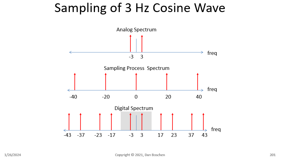
The first graphic shows the frequency spectrums involved in sampling a 3 Hz Sine wave with a 20 Hz sampling clock.

The top spectrum is the analog spectrum showing the Fourier Transform of a 3 Hz sine wave as two impulses in the frequency domain at +/- 3 Hz.

The middle spectrum shows the spectrum of the sampling process. Sampling in time is multiplying the analog waveform with a train of impulses. The Fourier Transform of a train of impulses in the time domain is a train of impulses in the frequency domain (we see a DC term, the 20 Hz sampling clock, and all the higher harmonics).

The bottom plot shows the digital spectrum that results as the convolution in frequency of the top two spectrums (multiplying in time is convolution in frequency). The convolution with impulses simply creates a copy of the analog spectrum wherever the spectrum appears in the Sampling Process spectrum. This results in the spectrum from $-f_s/2$ to $+f_s/2$ (First Nyquist Zone) being replicated in all higher Nyquist Zones. And for this reason we typically only need to show the digital spectrum from $-f_s/2$ to $+f_s/2$ as the rest is redundant. However visualizing this periodic spectrum extended to infinity can be helpful in understanding mixed signal (analog and digital) concepts. A key point to take away from this is the digital spectrum is periodic. What is in the first Nyquist Zone in the Digital Sepctrum must also be in the higher Nyquist Zones. Similarly anything introduced into the higher Nyquist Zones MUST be in the first Nyquist Zone (they are periodically all the same spectrum).

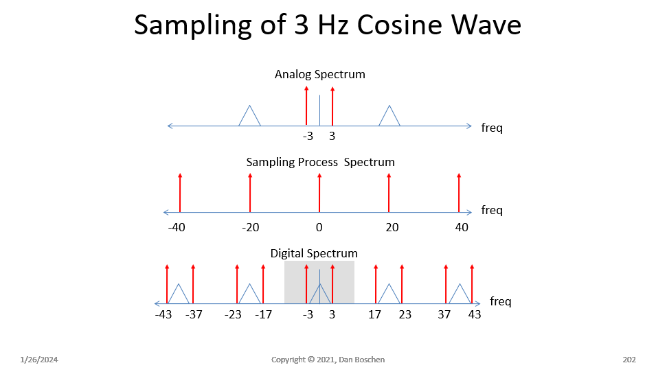
With that all in mind, I will now add another graphic below showing the same thing with an interference signal in the analog spectrum that is in the area of the sampling rate and not filtered with an anti-alias filter. This signal need not be periodic.

The same convolution process described above explains how the higher frequency spectrum aliases into the locations shown, and specifically how it can be an interference within our primary lower frequency spectrum of interest. The higher frequency spectrum must be filtered out prior to sampling to avoid this interference. An anti-alias filter is required.

Even when there is no apparent signals to filter out, the measured noise floor would (should) be amplified prior to sampling with the A/D converter, to be higher than the quantization noise contributions of the A/D, otherwise local quantization noise will dominate SNR degrading the measurement SNR. If an anti-alias filter is omitted, this amplified noise floor that exists in the bands that will alias into our bandwidth of interest will increase the overall noise floor also degrading the measurement SNR. (For the case of a sensitive radio receiver, this would be the receiver noise figure metric that would be significantly affected).