Design of digital filters with negative group delay

Question

I am currently working on digital filters that can predict my input signal(assume that input signal is bandlimited). In other words, I want my filter to have a flat magnitude response in bandwidth of interest (let's say, $0$ to $\pi/4$), as well as a constant and negative group delay in bandwidth of interest. Since I have to implement it, the order of the filter should be as low as possible.

I noticed that $H(s)=1+s\tau$ reaches all my requirements. However, transfering it to digital filter using bilinear transform will destroy its group delay response.

I wonder is there any methodology or something like a MATLAB toolbox to help me design such a filter? Or if anyone could provide a prototype?

Answer 1

Here is another version.

This is a tricky problem. Allpass filters clearly don't work here since the have a strictly monotonic decreasing phase, so the group delay is always positive. That means the best we can do is optimize over a limited frequency area.

A better choice are probably minimum phase filters. These can indeed have negative group delay. Here is why: the inverse of a stable minimum phase filter is also stable and minimum phase. The inverse has the negative group delay of the original filter, i.e.

$$\tau_g(\frac{1}{H[z]}) = -\tau_g(H[z])$$

The group delay tends to be negative on an upwards slope. An interesting choice are lowshelf filters. Here is an example of a lowshelf with a gain of -6dB, a center frequency of 4 kHz and Q of 1 sampled at 48 kHz. You have a group delay of about -1.1 samples and a fairly flat amplitude response up to about 1kHz or thereabouts.

Answer 2

The analog filter you came up with exemplifies the problem that one usually encounters when designing filters with negative group delay in a certain frequency band. The filter with transfer function $H(s)=1+s\tau$ is unstable, and its frequency response grows indefinitely towards high frequencies.

I have a neat solution for designing a discrete-time 1-step predictor, i.e., a filter predicting $1$ sample into the future. Clearly, such a filter must approximate a group delay of $-1$ sample in a certain frequency band. We can choose any frequency band, but let's assume that we care about low frequencies close to DC.

The design method is based on the fact that the optimal linear prediction error filter is a minimum-phase filter [1, 2]. If $P(z)$ is the linear prediction filter, the prediction error filter is

$$E(z)=1 - z^{-1}P(z)\tag{1}$$

Its output is the prediction error of the predictor $P(z)$. Note that if $P(z)$ approximates an advance of $1$ sample, i.e., $P(z)\approx z$, the output of $E(z)$ is approximately zero. Of course, a causal filter cannot closely approximate the transfer function $P(z)=z$ over the whole frequency band, but it can approximate an advance of $1$ sample in some specified band. Note that this approximation implies that in the specified band the group delay is close to $-1$ sample, and the magnitude is close to $1$.

In order to find such a prediction filter $P(z)$, we can choose a strictly minimum-phase filter $E(z)$ with a magnitude response that approximates zero in the band of interest, and with a limited magnitude response elsewhere, such that the approximation error doesn't grow without bounds outside the band of interest.

A good candidate for $E(z)$ is a Butterworth filter. If we're interested in a predictor for low frequencies, we need to choose a highpass filter for $E(z)$. From $(1)$ we see that we need to normalize $E(z)$ such that the first coefficient of its impulse response equals $1$. Then we can compute the prediction filter from $(1)$:

$$P(z)=z\big(1-E(z)\big)\tag{2}$$

I.e., if the normalized prediction error filter is given by

$$E(z)=\frac{\sum_{k=0}^Nb_kz^{-k}}{\sum_{k=0}^Na_kz^{-k}}\tag{3}$$

the transfer function of the predictor is

$$P(z)=\frac{\sum_{k=0}^{N-1}\big(a_{k+1}-b_{k+1}\big)z^{-k}}{\sum_{k=0}^Na_kz^{-k}}\tag{4}$$

This little Matlab/Octave script designs a 1-step predictor using this method:

n = 5; wc = .4;
[be,a] = butter( n, wc, 'high' );    % prediction error filter
be = be / be(1);                     % normalization
b = a( 2 : n+1 ) - be( 2 : n+1 );    % numerator of predictor
                                     % a = denominator of predictor

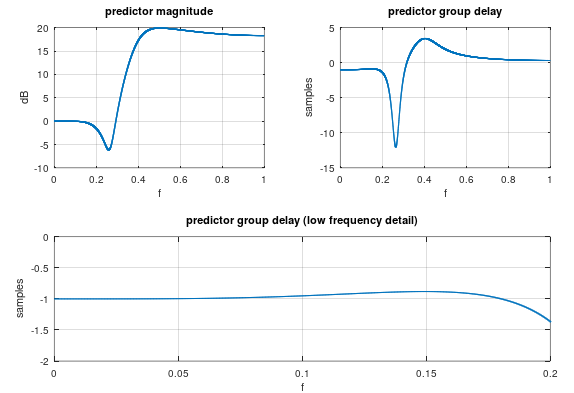
The figure below shows the result. The predictor has a flat magnitude of $0$ dB and a flat group delay of $-1$ sample at low frequencies, and the growth of the magnitude response outside the band of interest is limited.