1
$\begingroup$

I'm a DSP newbie trying to get into the field. Despite being able to use some of the MATLAB tools, I'm still not completely solid on some intuition of the frequency domain.

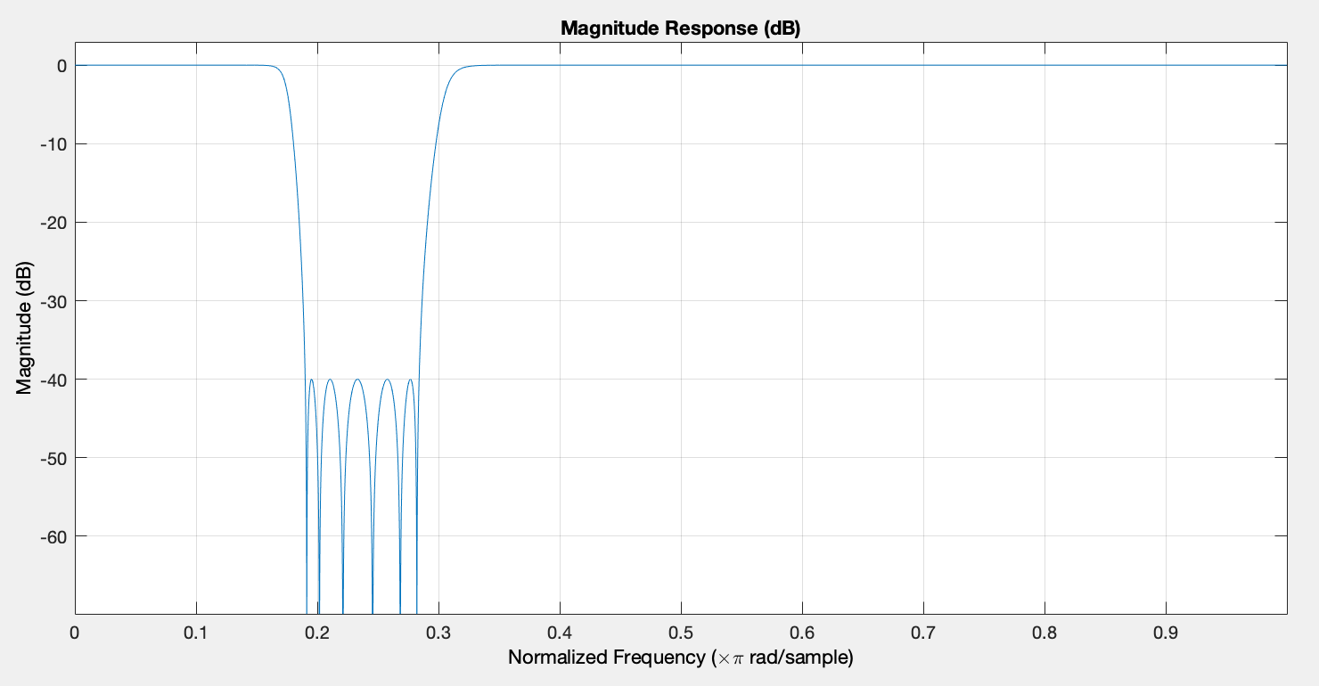
I've implemented a biquad Chebyshev type 2 filter in direct form II using design() and fdesign(), and cascaded an all pass filter before it to make sure the phase is approximately linear using iirgrpdelay()

enter image description here

Here are my filter coefficients. The cascade filter is made up of two stages; the first is an all-pass equalizing filter and the second is my band-stop filter.

Stage 1 SOSMatrix:

   0.381213874783434  -1.557955120504960   1.591776409857931   1.000000000000000  -0.978752487382327   0.239489586868207
   0.552531400073819  -0.022041931397907   0.944632862505602   1.000000000000000  -0.023333860458169   0.584916555420538
   0.208375162206942   0.338597008794322   0.403080816836635   1.000000000000000   0.840022632313836   0.516956286439685
   0.738077366524991   2.000000000000000   1.498774195719990   1.000000000000000   1.334423828293380   0.492454012507487

Stage 1 ScaleValues:

   0.260737099485881
   1.000000000000000
   1.000000000000000
   1.000000000000000
   4.222053367426932
   
Stage 2 SOSMatrix:

   1.000000000000000  -1.649455187829982   1.000000000000000   1.000000000000000  -1.104541883178642   0.913753853150600
   1.000000000000000  -1.264410719232027   1.000000000000000   1.000000000000000  -1.653222532296871   0.943601232271565
   1.000000000000000  -1.611538275581591   1.000000000000000   1.000000000000000  -1.117951080612895   0.785871033092721
   1.000000000000000  -1.329923547522389   1.000000000000000   1.000000000000000  -1.524529858509588   0.841251385596782
   1.000000000000000  -1.536278103762843   1.000000000000000   1.000000000000000  -1.372242531855038   0.762644118662937
   1.000000000000000  -1.433307330009434   1.000000000000000   1.000000000000000  -1.221557613144382   0.735502467713962

Stage 2 ScaleValues:
   
   0.954605779388083
   0.954605779388083
   0.901497869853696
   0.901497869853696
   0.873798810487316
   0.873798810487316
   1.000000000000000

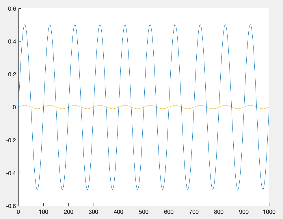
The frequency response looks according to the spec., but my input is coming out attenuated. I should put a legend here but the blue line is the input and yellow line the output.

enter image description here

Here's how I'm constructing my sinusoidal input; the amplitude is -6dB full-scale and its frequency is set to 0.01. My filter sampling frequency is 1MHz, and it's to my understanding that this sinusoid should be within the passband.

% Generate input
% input attenuation; <db> and <absolute value>
input_att_db = -6;
input_att_ab = 10 ^ (input_att_db / (-20));

% input sinusoid with angular frequency w0 for L samples
f0 = 0.01;
w0 = 2 * pi * f0;
L = 1000;
n = 0:L - 1;
input = sin(w0 * n) / input_att_ab;

I'm then just calling the filter as if its a function. I named my filter cas short for "cascade".

outputi = cas(input);
plot(n, outputi)

Is this normal? If not what could I be doing wrong? Any pointers would be much appreciated!

$\endgroup$
9
  • $\begingroup$ Generally your code looks ok. Your signal frequency isn't where you think it is but it's still in the pass band. so this unexpected behavior. $\endgroup$
    – Hilmar
    Commented Dec 8, 2022 at 11:25
  • $\begingroup$ It's hard to tell as long as we don't know what exactly cas() is doing. $\endgroup$
    – Matt L.
    Commented Dec 8, 2022 at 12:22
  • $\begingroup$ @MattL. cas() is my filter, short for "cascade"; I saw it used this way in this matlab documentation for biquad iir filters. mathworks.com/help/dsp/ref/dsp.biquadfilter-system-object.html It's down in the first example, could I be messing up here? $\endgroup$
    – Chris H.
    Commented Dec 8, 2022 at 14:16
  • $\begingroup$ @Hilmar Any idea where I could be messing up? Or is there anything else I could provide to help you diagnose? $\endgroup$
    – Chris H.
    Commented Dec 8, 2022 at 14:20
  • $\begingroup$ @ChrisH.: I don't know but I don't see any other possibility where things might have gone wrong. $\endgroup$
    – Matt L.
    Commented Dec 8, 2022 at 14:22

2 Answers 2

2
$\begingroup$

You can use the filter coefficients and scaling values to check whether the filters work as expected. Assuming that your SOS matrices are stored in the variables sos1 and sos2, and that the corresponding scaling values are in the arrays scale1 and scale2, the output can be computed by

g1 = prod(scale1);
g2 = prod(scale2);
y = g1 * sosfilt(sos1,input);
y = g2 * sosfilt(sos2,y);

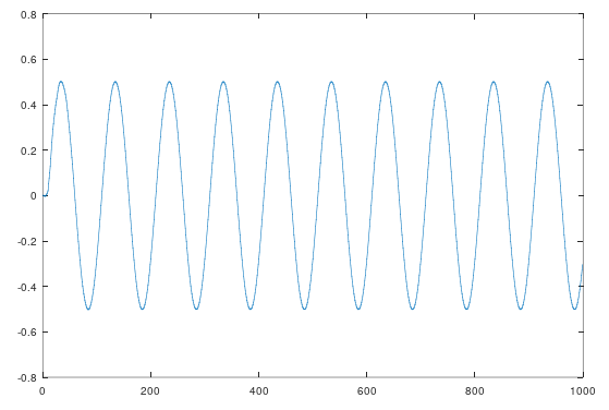
Using your input signal, I get the following plot for the output signal:

enter image description here

This is exactly what one would expect. This means that the additional scaling that you see must happen somewhere in the blackbox cas(). The filters themselves do what you intend them to do.

EDIT:

The delay of a sinusoidal input signal is determined by the phase delay of the filter, not by the group delay. Phase delays of concatenated filters simply add up. The phase delay of a filter with frequency response $H(e^{j\omega})$ is given by

$$\tau_p=-\frac{\textrm{arg}\big\{H(e^{j\omega})\big\}}{\omega},\qquad\omega\neq 0$$

where $\textrm{arg}\big\{H(e^{j\omega})\big\}$ is the filter's phase response.

You can compute the phase delay at the input frequency $\omega_0$ using the following Matlab/Octave code:

[b1,a1] = sos2tf(sos1,g1);
[b2,a2] = sos2tf(sos2,g2);
H1 = polyval( b1, exp(1i*w0) ) / polyval( a1, exp(1i*w0) );
H2 = polyval( b2, exp(1i*w0) ) / polyval( a2, exp(1i*w0) );
tp1 = - angle(H1) / w0;
tp2 = - angle(H2) / w0;
tp1 + tp2    % total phase delay

The total phase delay at the input frequency $\omega_0$ is about $9.4$ samples, which agrees with your observation.

Note that not only the allpass filter but also the bandstop filter contributes to the phase delay

$\endgroup$
5
  • $\begingroup$ The amplitude is fixed now, thank you! But there seems to be a delay of around 9 samples compared to the input; is this expected for iir filters or filters in general? I thought it would be correlated to the group delay specification I set for the all pass filter to meet, and to my surprise the more lax my group delay spec. is the smaller the delay at the output. Group delays within [4, 7, 10, 13, 16], correspond to output delays [20, 19, 9, 2, 3]. $\endgroup$
    – Chris H.
    Commented Dec 11, 2022 at 11:54
  • $\begingroup$ @ChrisH.: I'll edit my answer to address the delay. What was the issue with the amplitude scaling? $\endgroup$
    – Matt L.
    Commented Dec 11, 2022 at 12:29
  • $\begingroup$ I feel stupid even admitting this, but when one calls a dsp.FilterCascade as a function, what matlab actually does is return the filter's step function. The "input" becomes the time vector the step response is evaluated at. It's even noted in the documentation page I was referencing; "Note: If you are using R2016a or an earlier release, replace each call to the object with the equivalent step syntax. For example, obj(x) becomes step(obj,x)." $\endgroup$
    – Chris H.
    Commented Dec 11, 2022 at 13:14
  • $\begingroup$ @ChrisH.: Ok, strange ... If you look at my updated answer you'll see that a delay of about 9 samples at the input frequency is exactly what one would expect. $\endgroup$
    – Matt L.
    Commented Dec 11, 2022 at 13:22
  • $\begingroup$ That makes sense, thank you for thorough response. I plotted grpdelay(cas)(cas being my filter), and the point at w0 ~= 0.011 corresponds to a delay of ~9.38, which also corroborates your result. $\endgroup$
    – Chris H.
    Commented Dec 12, 2022 at 8:56
0
$\begingroup$

Either

1.- Aliasing is taking place, because chosen fs sampling frequency too low, let's assume it's not the case

or

2.- Your filter stop-band and the input signal are on same frequency because the displayed fvtool response is not frequency in Hz but f/fs no units.

The plotted 'frequency' in the response displayed in the question argued as 0.01Hz is not actually 0.01Hz but f1/fs = 0.01 .

3.- Since the actual input carrier frequency is not mentioned why don't we try the following

bandstopSpecs = fdesign.bandstop('N,Fp1,Fst1,Fst2,Fp2,C',60,9.6e3,12.8e3,22.4e3,25.6e3,128000)

bandstopSpecs.Passband1Constrained = true;

bandstopSpecs.Apass1 = .1;

bandstopSpecs.Passband2Constrained = true;

bandstopSpecs.Apass2 = .1;

bandstopFilt = design(bandstopSpecs,'Systemobject',true)

fvtool(bandstopFilt)

3.1.- this is fvtool response in Hz

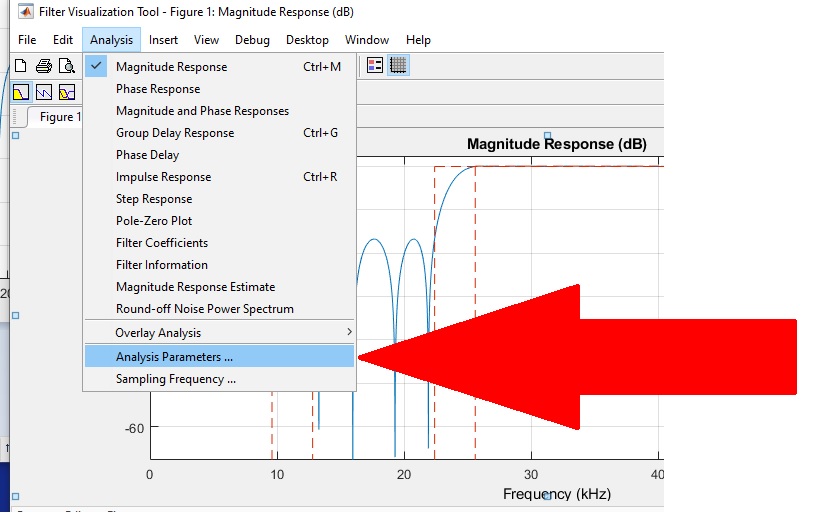
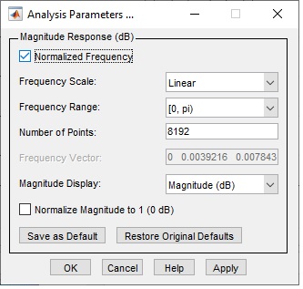
Now pull down the Analysis menu and choose Analysis Parameters

enter image description here

In this window tick the normalized box option:

enter image description here

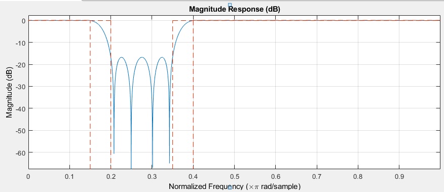
3.3.- Observe that now the x-axis displays the same

'f x pi radian / SAMPLE'

shown in the question

enter image description here

The x-axis is no longer in Hz , is it ?

The question originator assumed that the x-axis readings are Hz

4.- I suggest to do what we would do with a conventional desktop set-up :

Shift up and down the generator frequency and observe the filter output.

Rewording : Try sweeping input carrier f1 from as low as possible up to let's say fs/2 to avoid Aliasing.

One should then see at what frequencies the stop band really takes place.

$\endgroup$
2
  • 1
    $\begingroup$ The input frequency is definitely not in the filter's stopband. $\endgroup$
    – Matt L.
    Commented Dec 11, 2022 at 12:46
  • $\begingroup$ Hi Matt, thanks for the comment. Please read my reworded answer. $\endgroup$ Commented Dec 13, 2022 at 21:40

Your Answer

By clicking “Post Your Answer”, you agree to our terms of service and acknowledge you have read our privacy policy.

Not the answer you're looking for? Browse other questions tagged or ask your own question.