Mapping of Classic Filters for Digital Filter Design

Question

Of the four classic analog filter types: Butterworth, Chebyshev, Elliptic and Bessel- are any of these relegated to obsolescence for purposes of digital filter design in comparison to optimized algorithms such as least squares (firls), Parks-McClellan (firpm or remez), maximally flat (maxflat), etc?

(NOTE: This question is not in regards to the common and useful application of simple IIR structures for loop filters, leaky accumulators, notch filters, or in regards to using optimized IIR structures as direct digital designs. My question is specific to the approach of designing higher performance low pass, high pass or band pass structures specifically by copying the analog classics-- there may be actual utility in doing this beyond my current narrow view).

I have been taught (fred harris and others) to avoid the trap of "copying the analog" given those techniques with the classic types are limited to what we can feasibly do with a relatively low number of inductors and capacitors, while in the digital world we have the full power of the underlying mathematics and scalability with simple delays and multiplies (and non-linear commutators for multi-rate design resulting in very efficient FIR structures). My use of the mapping from s to z (as was common prior to the late 1960's given the wealth of knowledge in analog filter design) is mostly limited to simulation and modelling of existing analog filters, but not for the creation of new digital filters for common low pass, high pass and band pass structures.

That said I could be missing succinct and good practical applications beyond modelling and simulation where "copying the analog" would result in the better solution.

The best answer will list out applications for common low pass, high pass and band pass filters designs (not notch filters where an IIR would certainly rule) that the optimized algorithms specific to FIR filters (including optimized multi-rate structures) cannot possibly surpass in performance, for any of the class filter types (or prove why the optimized algorithms are always preferred if that is the case). A second best answer if it's only an assumed statement or suspicion is to at least demonstrate a specific case of such a mapped filter to allow for testing against an "optimized" direct digital solution.

Answer 1

and simulation where "copying the analog" would result in the better solution.

That' missing the point a bit. It's not that one cares much about matching or copying the "analog" but that digital IIR filters have some very nice and useful properties.

For example in audio, IIR filter are very common place and I use Butterworths on a daily basis.

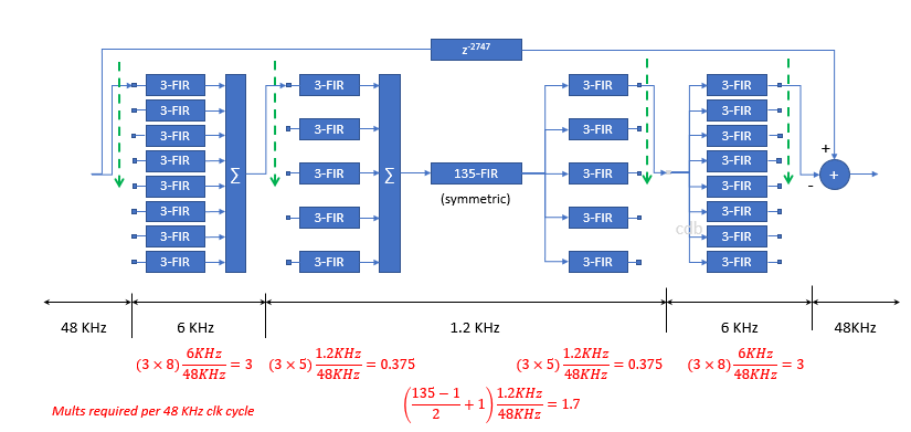
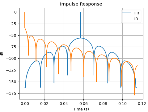
The most straight forward reason is simply filter length. To do anything meaningful at 40 Hz when your sample rate is 48 kHz, an FIR filter needs to be thousands of taps long. In some cases you can use multi rate filters to implement this very efficiently, but I'm not sure if this is universally applicable. Another possible option are FFT based filter (overlap add, etc.) but that presents a non-trivial trade off between latency and efficiency.

If you stick with linear phase filters, the latency quickly gets prohibitively large and you loose causality. Technically you can turn any linear phase FIR into a minimum phase FIR by simply inverting the zeros that are outside the unit circle, but that's numerically awkward procedure at high orders.

The human ear is also fairly insensitive to monaural phase distortions (e.g. minimum phase) as long as its causal. However, it's very sensitive to pre-ringing, so linear phase filters can be perceptually problematic.

A more "philosophical reason" is that the human auditory uses more or less logarithmic frequency axis and IIR filters are much more natural fit for this. For example, an IIR octave bandpass filter at 8kHz looks exactly the same as one at 125 Hz (other than the center frequency). The FIR filters would be dramatically different.

IIRs are great for cross overs: odd order Butterworth low pass and high pass filters sum to a flat frequency response (although it's typically an all pass). For even order, you can use Linkwitz Riley filters (which are based on Butterworths). You could use linear phase FIRs instead, but again you run into latency and causality problems.

It's also very easy to do things like real time adjustable high and low pass filters: It's very easy to design Butterworth filters on the fly or to simply table up the pole locations and interpolate. Filter order always stays constant and you are guaranteed to have the same slope & shape.

In other words: turn on any loudspeaker in your home and you will be hearing plenty of Butterworth & friends in action :-)

Example 1

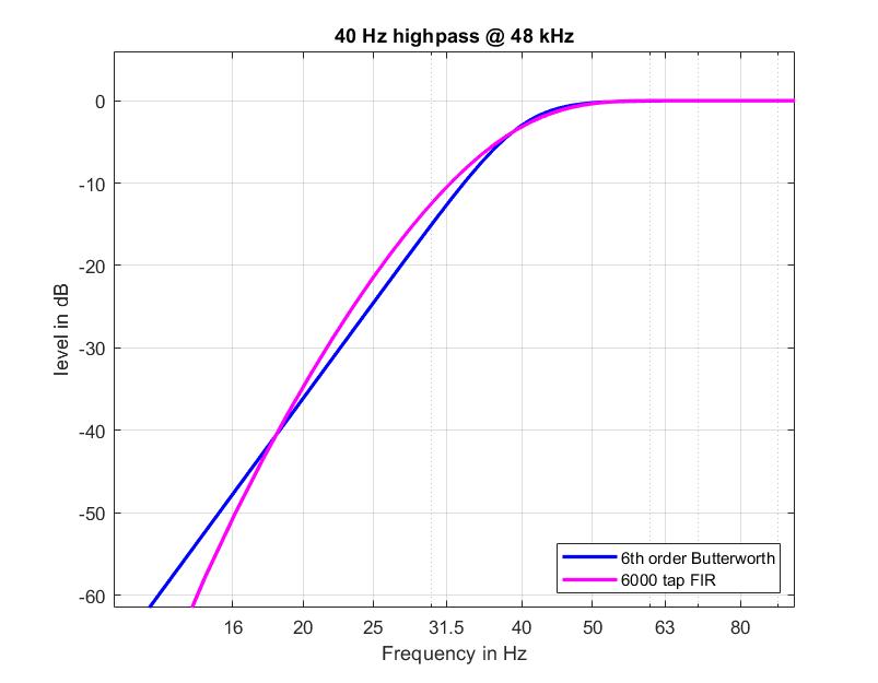
This just a very simple highpass you would in any garden variety active speaker. 40 Hz sampled at 48 kHz. I designed both a Butterworth Highpass and a "matching" FIR using firls() . Matching was done manually so they kind of look the same. I needed about 6000 taps on the FIR filter to get it in the ballpark

% IIR
[z,p,k] = butter(6,40*2/48000,'high');
%FIR
h=firls(6000,[0 10 65 fs/2]*2/fs,[0 0 1 1])';

Transfer function look like this.

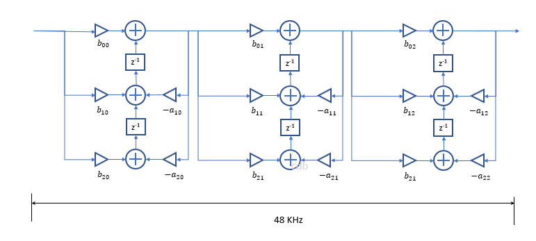
To me it seems like the FIR is very much inferior in terms of latency, memory footprint. A 6th order BW has only 13 coefficients and 6-8 state variables. You can reduce this even further by leveraging that the zeros are all at $z = 1$.

Example 2:

This one is expands on the previous example by making the cutoff frequency of the high pass adjustable in real time. This creates a "sliding high pass" filter which is commonly found in sealed smart speakers. I tried to make requirements realistic, as you would find them in real products.

The Butterworth allows an extremely efficient implementation with no audible artifacts, no inherent latency, very low memory footprint and very low CPU consumption.

%% Script to implement a sliding high pass filter, that can be adjusted on the fly
% This type of "sliding highpass" is typically used in smart speakers with a
% "closed box" topology to control trasnducer excursion at high output
% volume
%
% Requirements:
%  - sample rate: 48 kHz
%  - frame size: 128 samples
%  - cutoff frequency varies from 40 Hz to 100 Hz
%  - highpass slope: 36 dB/octave. In other words level at half the cutoff
%      frequency should be <= -36 dB
%  - Level at cutoff frequency not less than -3dB
%  - passband ripple: < .01 dB above 200 Hz (where spectral perception is
%                      more sensitive)
%  - cutoff frequency is updated once per frame
%  - no additional latency
%  - smooth updating filter, no pops or clicks  
%
% Implementation
%  - 6th order butterworth
%  - pole location and filter gain as a function of frequency are 
%    approximated as a polynomial fit. At these low frequencies, a linear
%    fit (1rst order polynomial) works perfectly.
%  - The filter coefficients are calcuated once per frame based on the
%    current cutoff frequency
%  - Filter is implemented as cascaded second order sections in Direct Form
%    I. For Direct Form I, the state variable are simply the inputs and
%    outputs, so updateing the filter deosn't create a discontinuity in the
%    state variables.
%
%  Test
%  - input signal is a 50 Hz sine wave, low frequency sine waves are very
%    sensitive to artifacts
%  - cutoff frequency input is a mixture of step function, up and down sweeps
%    and uniformly distributed random numbers between 40Hz and 100Hz
%


%% Table up the poles and the gain of the filters, perform polynomial fit
ord = 6;
fs = 48000;
fr = (40:.1:100)';
nfr = length(fr);
p0 = cell(nfr,1);  % pole locations
k0 = zeros(nfr,1); % filter gains
for i = 1:nfr
  [z,p,k] = butter(ord,2*fr(i)/fs,'high');
  p0{i} = p(imag(p)>0);
  k0(i) = k;
end
p0 = [p0{:}].'; % convert cell array to regular array

%% do a simple linear for poles and gains
% we fit the real part and the gain in (1-x) since they are very close to 1

ppPoles = cell(3,2);
for i = 1:3
  ppPoles{i,1} = polyfit(fr,1-real(p0(:,i)),1); % 1 minus real part
  ppPoles{i,2} = polyfit(fr,imag(p0(:,i)),1); % imginary part
end

% and the gains in 1-k
ppGain = polyfit(fr,1-k0,2);

%% test the polyfit, calculate the resulting transfer functions at a few
% frequencies
frTest = 40:10:100;
nfrTest = length(frTest);
nFFT = 16384*2;
d0 = zeros(nFFT,1); d0(1) = 1;
fy = zeros(nFFT,nfrTest);
sos = zeros(ord/2,6);
sos(:,1) = 1; sos(:,2) = -2; sos(:,3) = 1;
for i = 1:nfrTest
  f =  frTest(i);
  for ip = 1:3
    x = 1-polyval(ppPoles{ip,1},f); % real part
    y = polyval(ppPoles{ip,2},f); % imginary part
    sos(ip,4:6) = [1 -2*x x^2+y^2];
  end
  k = 1-polyval(ppGain,f);

  fy(:,i) = fft(k*sosfilt(sos,d0));
end
% this checks out fine

%% Real time part, preperation
frameSize = 128;  % frame size
frameRate = fs/frameSize; % number of frames per second

% let's do 10 seconds but an integer number of frames
nx = 10*fs;
numFrames = floor(nx/frameSize);
nx = numFrames*frameSize;

% build a test signal: 50 hz sine wave
xin = sqrt(.5)*sin(2*pi*(0:nx-1)'*50/fs); % 50 Hz sine wave at -3 dB
% build control frequency signal, one frequency per frame
frInput = 40*ones(numFrames,1);
% let's do a bit of rectangular switching plus some random stuff
t = (1:frameRate);
frInput(frameRate+t) = 100;
frInput(3*frameRate+t) = 70;
% up and down sweep
frInput(5*frameRate+t) = linspace(40,100,frameRate);
frInput(6*frameRate+t) = flip(linspace(40,100,frameRate));
% some random numbers for good measure
frInput(7*frameRate+1:end) = 40+60*rand(3*frameRate,1);
% 
% in order to smooth the very aprupt frequency transitions in the test
% vector, we smooth the frequency input with a time constant to 30ms
timeConstant = 0.03;
frSmooth = exp(-1./(timeConstant*frameRate));
frCurrent =40;

%% Real time over all frames
% we implement this as driect form I so the states are always guaranteed to
% be continous
signalState = zeros(2,4);  % filter state, we need total of 8
freqState = frInput(1); % cutoff frequency states
xout = 0*xin; % initialize output
t = 1:frameSize; % time vector
t0 = 0;  % current time
yy = [xout xout xout];
for iFrame = 1:numFrames
  % get frequency input and apply smoothing
  frCurrent = frSmooth*frCurrent + (1-frSmooth)*frInput(iFrame);
  % calculate filter gain, grab input and scale it
  k = 1-polyval(ppGain,frCurrent);
  y = k*xin(t0+t);

  % over all biquads
  x1 = signalState(1,1); % grab input state for the first biquad
  x2 = signalState(2,1);
  for iPole = 1:3
    % calculate the filter coeefficents
    pReal = 1-polyval(ppPoles{iPole,1},frCurrent); % real part
    pImag = polyval(ppPoles{iPole,2},frCurrent); % imaginary part
    a1 = -2*pReal;                % filter coefficient "a1"
    a2 = pReal*pReal+pImag*pImag; % biquad coefficient "a2"
    % grab the output state
    y1 = signalState(1,iPole+1);
    y2 = signalState(2,iPole+1);
    % inner loop. Here efficieny is the most important
    for i = t
      x0 = y(i);  % get input sample
      y0 = x0-2*x1+x2-a1*y1-a2*y2; % DF1 Butterworth stage
      % update state
      x2 = x1; x1 = x0;
      y2 = y1; y1 = y0;
      y(i) = y0; % write output
    end % end sample loop
    % save the output state of this stage
    signalState(1,iPole) = x1;
    signalState(2,iPole) = x2;
    % grab the input state for the next stage
    x1 = signalState(1,iPole+1);
    x2 = signalState(2,iPole+1);
    % now write the output state
    signalState(1,iPole+1) = y1;
    signalState(2,iPole+1) = y2;

    yy(t0+t,iPole) = y;
      
  end % end poles/stages
  % write output
  xout(t0+t) = y;
  t0 = t0 + frameSize;
  
end % end frame

plot(xout);

Answer 2

I'm convinced that depending on the problem we're trying to solve, we can and should use both approaches: the transformation of classic analog filter designs, and the direct design in the digital domain using optimization methods. Note that the properties of the classic designs are very restricted: piecewise constant desired magnitude responses, minimum-phase, and optimality that is defined as maximal flatness (Butterworth) or minimum amplitude approximation error (Cauer = elliptic), or a combination of the two (both types of Chebyshev). If anything else is desired, then we need to resort to other methods.

But if we're content with a simple design with just (constant gain) passbands and stopbands, if we don't care about the phase response, and if the two above mentioned optimality criteria fit our purposes, then nothing can beat a minimum-phase IIR filter derived from the classic analog prototypes. Why is this the case? Well, because these filters are optimal according to the chosen criteria. By definition, there is no lower order filter that can do the job as well, and consequently, such a filter results in the most efficient implementation. We also shouldn't forget that the design is extremely simple, just based on formulas. Optimization methods for IIR filter design are still problematic because the design problem is highly non-linear, and there is no guarantee that we can find the global best solution. We always find some solution - a local optimum - but that might not be good enough.

If - as suggested in your question - we were to choose FIR filters as solutions to all filtering problems, then the design would be easier than in the case of IIR filters, because we're basically just dealing with well-researched polynomial approximation. However, note that most efficient FIR filter design methods result in linear-phase filters. Such filters introduce a huge delay if high orders are required. That delay may be prohibitive in some applications. Moreover, if high quality magnitude approximations are required (e.g., almost constant passbands, very high stopband attenuation), then the resulting high filter orders also result in large implementation complexity in terms of memory as well as computations.

There are methods for non-linear phase FIR filter design but they are less widely available and often less efficient. Moreover, if we don't care about the phase, we do not want to specify any non-linear desired phase response - as is necessary for those routines - but we just want to specify a magnitude response and let the phase take care of itself. In such cases, a minimum-phase design would be required. However, even though there are methods for minimum-phase FIR filter design, these methods are not efficient and not numerically robust, and hence they are impractical for high filter orders.

Summarizing, in all cases where the application requires more flexibility than the classic analog filter designs can offer, we need to use optimization methods anyway, and more often than not, we would choose FIR filters due to their many advantages over (numerically designed) IIR filters (e.g., relative ease of design and implementation, absence of limit cycles, inherent stability). But if the problem can be solved with classic designs, I see no reason to use anything else, because the classic designs result in reliable and very efficient filters.

As a final note, I haven't mentioned Bessel filters yet. These are the only ones I would consider obsolete as prototypes for digital filter design. The reason is that their maximally flat group delay property doesn't carry over to the digital domain due to frequency warping of the bilinear transform. If maximally flat group delay is desired, we need to formulate the problem directly in the digital domain. This has been done and solved by Thiran:

Thiran, J. P. (1971-11-01). "Recursive digital filters with maximally flat group delay". IEEE Transactions on Circuit Theory. 18 (6): 659–664.

---

EXAMPLE:

I've designed a $15$th order elliptic low pass filter with a passband ripple of $0.5$ dB and a stopband attenuation of 100 dB. The design criterion of an elliptic filter is minimum deviation from the desired constant magnitude response. This corresponds to the design criterion used by the Parks-McClellan algorithm for linear-phase FIR filters. It turned out that in order to satisfy the same requirements on the magnitude response, a linear-phase filter of order $667$ is required. The magnitude responses of the two filters are shown below:

The maximum passband and stopband approximation errors are virtually identical. Note, however, that for practical purposes there are still some noticeable differences between the two filters. First of all, due to the few stopband ripples of the IIR filter, the stopband attenuation is much greater in several frequency bands than for the FIR filter. Second, the transition from the passband to the stopband is much sharper for the IIR filter. This is a simple consequence of poles relatively close to the unit circle. Of course, such poles can pose a serious problem in a fixed-point implementation. Another difference between the performance of the two filters is the pre-ringing of the linear-phase FIR filter, which is undesirable in audio applications.

Finally, the linear-phase FIR filter obviously has a much larger delay than the minimum-phase IIR filter. Its group delay is constant ($667/2=333.5$ samples), whereas the group delay of the IIR filter is frequency-dependent. The average passband group delay of the IIR filter is approximately $20$ samples (see figure below). If linearity of the phase is not a requirement, we might as well use a minimum-phase FIR filter with the same magnitude as the linear-phase FIR filter. I explain the computation of that suboptimal minimum-phase filter in this answer. As shown in the plot below, the group delay of the minimum-phase FIR filter is very similar to the group delay of the IIR filter.

Concerning complexity, it is obvious that the $15$th order IIR filter is much cheaper to implement than the corresponding FIR filter of order $667$.

Answer 3

How to Massively Reduce the Resource Requirements in FIR Filter Approach

The two answers provided by Matt and Hilmar are both excellent and provide great insight in answering the question. I am favoring Hilmar's answer as correct given that it both touches on and demonstrates the salient points quite well, although I am not yet convinced in the efficiency claims that he has provided as I will detail here.

FIR of Hilmar's Filter with 8.45 Multipliers per Clock Cycle

What I am showing below I have not been able to do with Matt's filter due to the combination of his choice of signal bandwidth and tight transition width (I wouldn't be surprised if there are equivalent tricks that can be done in that case, but I can't see the path to doing that yet). However, I was able to reduce Hilmar's implementation as a least squares FIR filter significantly. Hilmar highlights many other advantages that makes his implementation compelling for certain applications, but I do want to clear up the misconception that the FIR filter would require thousands of multipliers on every clock cycle. The reason is multi-rate signal processing---and the advantages that can be gained by running selected portions of the signal processing required at the lowest rate possible.

Comparison of Filtering Performance

First I will highlight the comparative results of Hilmar's IIR filter to my FIR filter implementation. Hilmar didn't detail a requirement, but I used a 16 bit 48 KHz audio dynamic range of 100 dB, (stop band consistent with what Matt had used in his post).

Below shows the Log Frequency plot of the transition band, consistent with the plot in Hilmar's post, except with my version of his IIR and FIR implementations.

And below is a quad chart similar to Matt's presentation but again for my version of Hilmar's IIR and FIR filters. For both filter implementations I used 28 bit coefficient quantization to include possible quantization effects and found that 28 bits was required for both in order to not deviate at this scale shown from the same floating point result:

6th Order 40 Hz HPF IIR Implementation

Starting with what I think is the equivalent of Hilmar's implementation; below are the 2nd order bi-quad coefficients I determined for a 6th order Butterworth IIR filter, quantized to 28 bits and normalized to reduce the number of multiplications required to 9 (11 total, but two only require bit-shifts). Notably, all of these multiplications are running at 48 KHz!

[[ 0.98993582 -1.97987163  0.98993582  1.         -1.98990852  0.98993579]
 [ 1.         -2.          1.          1.         -1.99259523  0.99262254]
 [ 1.         -2.          1.          1.         -1.99726595  0.99729332]]

Below is a block diagram showing the implementation of this IIR approach in case further simplifications can be identified. My preference for FPGA implementation is to use this transposed direct form 2 representation shown since it avoids adder trees and allows for running an implementation at the highest rate possible before running into timing delay issues (however this is certainly not an issue in a 48KHz audio filter).

5533th Order 40 Hz HPF FIR Implementation

Thanks to amazing power of decimation and interpolation techniques, we CAN run the core filtering operation at the lowest rate possible resulting in a significant reduction in multiplier operations per clock cycle - leading to minimizing resources and, significantly, power dissipation (which is directly proportional to clock rate; $P=CV^2f$). Certainly what we give up is memory requirements as I will detail, and overall delay and for those reasons we may favor the IIR approach Hilmar suggested, but it doesn't appear that we would actually require 1000s of multipliers on every clock cycle. The main point of the block diagram below is that with creative decimation and interpolation techniques, we have moved a significant amount of the processing to operate at 1200 Hz instead of 48KHz! The total number of real 28 x 16 multiplications required on each 48 KHz clock cycle is computed in red.

The above block diagram is functionally bit for bit equivalent to a 5534 tap linear phase FIR filter running at 48 KHz which would require 2217 multiplications per clock cycle:

What I had done here is implemented a least squares linear phase low pass complementary FIR filter using polyphase decimators: First I decimate by 8 to 6 KHz using a 24 tap decimation filter (reduced to 3x8 polyphase such that only 3 multipliers are used on each 48 KHz clock cycle. This is then followed with a 15 tap decimation filter reduced to a 3x5 polyphase to decimate 6 KHz samples down to the 1.2 KSps rate. Then at this signficantly lower rate, I implement a 40 Hz low pass filter using a 135 tap linear phase least squares FIR filter. The signal is then interpolated using the same filter coefficients as used in decimation back up to the 48 KHz rate. Because the filter was implemented as a linear phase filter (which we cannot do with an IIR), I was able to convert this to a high pass by simply subtracting the signal from "a wire" or in this case a 2747 sample delay, which is the group delay of the filter (57 ms). So if this delay was a concern, or the memory required to hold the 2.7K samples, the IIR as Hilmar presented would be a compelling option.

Impulse Response

Below shows the impulse response for the two implementations, on a log scale of the magnitude to highlight the differences. Here we see the dreaded "leading echoes" of a linear phase FIR filter, which I understand from RBJ, Hilmar and other audiophiles is pure evil in the audio world. Note how in both Matt's and Hilmar's implementations that there are both no leading echoes and substantially less overall delay with the IIR filter approach.

This was a first cut of the decimation/interpolation approach to show a true comparison of FIR vs IIR filters. The resource requirement can likely be further reduced with different combinations or further reductions in clock rate (certainly we could run the inner FIR at 200 or even less to get a 40 Hz high pass!). We could also potentially do this with an minimum phase FIR with decimation / interpolation but then we lose the nice feature (in Hilmar's case) of being able to convert a low pass to a high pass by simply subtracting a delay. The work to match the frequency selective delay of a minimum phase filter for subtraction may be quite challenging. The point that this is a linear phase FIR is important to realize the low pass to high pass for this example as done.

Resource Requirement Summary

A summary of the resource requirements for the FIR is as follows:

• 8.45 real multiplications per 48 KHz clock cycle

• 13.35 real additions per 48 KHz clock cycle

• 2747 x 16 bit RAM for input signal

• (3x8 + 3x5 + (135-1)/2+1 ) = 104 x 24 bit RAM for coefficients

• 207 x 16 bit RAM for filter state storage

So for cases when memory and 57 ms delay is not an issue, and power dissipation and multiplier resources are of upmost concern- the FIR approach offers a very compelling option even for this challenging implementation Hilmer had suggested (features of dynamic tunability are also easily done given that is completely covered by the response of the core 135 tap FIR filter used). This was a first draft and I am confident if needed the resource requirement could be significantly reduced further given that we are still running a filter with a 40 Hz cutoff at a relatively high 1.2 KHz rate. What may continue to be an issue that the FIR approach cannot easily eliminate but minimize is the leading echoes. This was all very interesting and I greatly appreciate both Matt's and Hilmar's contributions and thoughts.

For the complete details on multirate techniques such as this, see fred harris' recently published 2nd edition of Multirate Signal Processing (I cannot find any copies of the first edition right now for anything less than $500).