It is common knowledge that the duration time samples are collected is inversely proportional to the width of the main lobe in the Fourier domain. The simple example is the rectangular pulse in time whose Fourier transform is the sinc function. The width of the rectangular pulse is inversely proportional to the position of the first zeros of the corresponding sinc function.
As a result, if you desire to decrease the width of the main lobe in the frequency domain, you should take additional samples in the time domain.
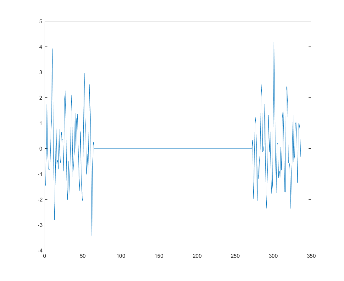
I am working on a project wherein I can collect only a certain number of sequential samples, let's say $N$. After I collect $N$ time domain samples, I must wait a certain duration before I can collect another set of $N$ samples. Let's define the number of missing samples in the "gap" as $M > N$. As a result, the time samples might look something like the following: 
There are 3 scenarios to consider:
- "Sample sets": two sets of samples over the time indices $n \in [0, N-1] \cup [M + N, M + N - 1]$
- "Aggregated Samples": single sets of samples over the time indices $n \in [0, 2N - 1]$
- "Fully Sampled": single sets of samples over the time indices $n \in [0, 2N + M - 1]$
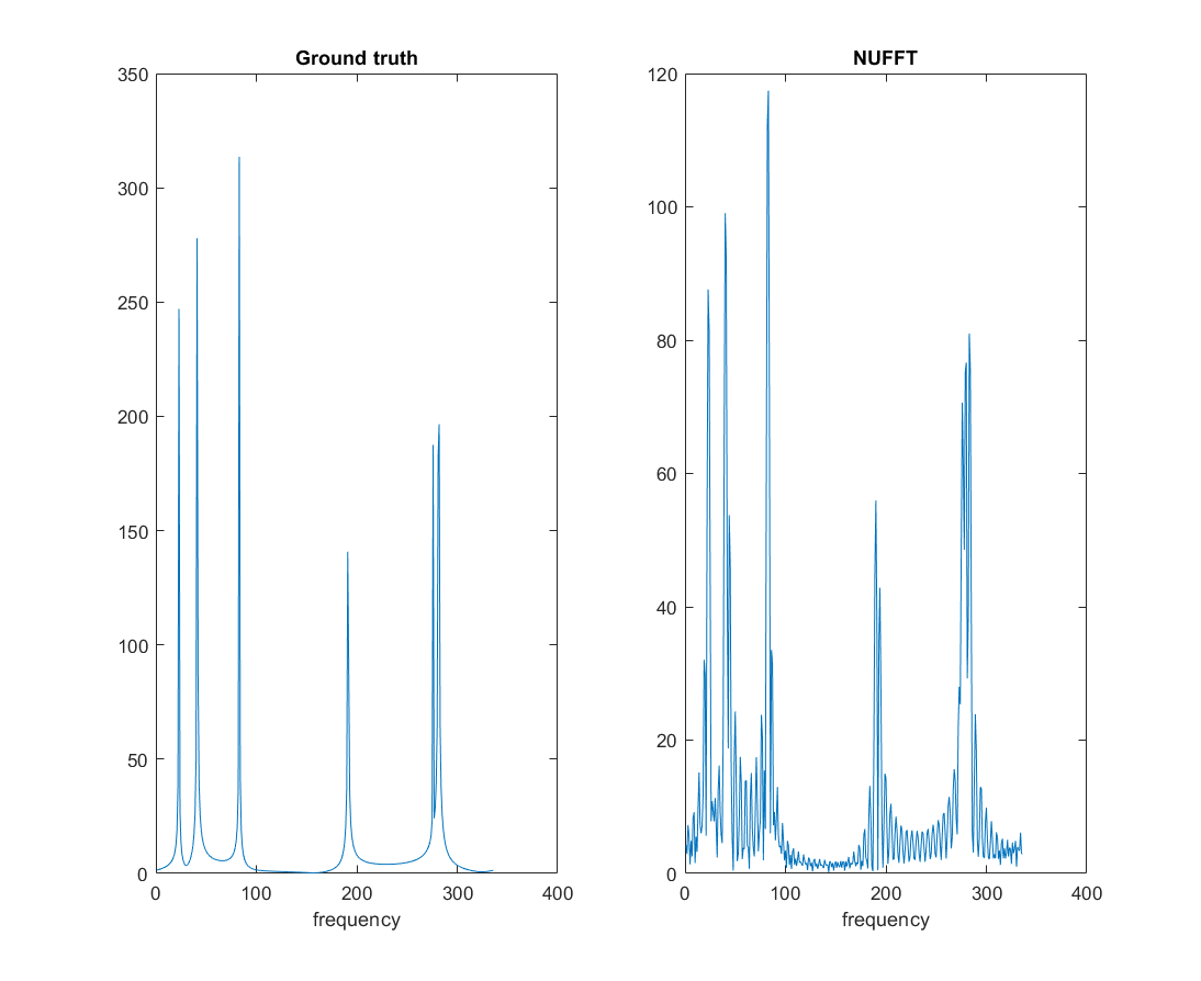
Considering the scenario 1, shown in the first figure, I have collected $2N$ samples but there is a spacing between them. My goal is to recover the Fourier transform of either scenario 2 or 3. In either case, we should see an reduction in the main lobe width in the frequency domain. However, because of the large gap between sample sets in scenario 1, if I use a nonuniform fast Fourier transform (NUFFT computed in MATLAB) or fill the gap with zeros (which is mathematically identical to the NUFFT in this case), the resulting grating lobes dominate the spectrum. Below is a comparison of scenario 3 and scenario 1. As evident in the figure, the frequencies that are closely spaced are considerably distorted due to the finite size as compared with the ideal case. A similar phenomenon can be observed if we were to compare scenarios 2 and 1.
If I were to recover the frequency domain representation of scenario 3, I essentially would be interpolating between the sample sets. If I were to recover the frequency domain representation of scenario 2, I essentially would be moving the second sample set next to the first and resolving the phase difference between the set of samples that would exist at $n \in [N, 2N -1]$ and the set of samples I have which were taken at $n \in [M + N, M + N - 1]$.
Some other notes:
- The signal I am sampling consists of a sum of sinusoidal signals each of which have different frequencies and are likely to be close to each other in frequency, but the number of different components is typically large $>> N$.
- For various reasons, I cannot use an autoregressive (AR) method, MUSIC/ESPIRIT/etc. method, Prony's method, or matrix pencil algorithm
- I have attempted various compressed sensing (CS) methods with limited success as my samples are taken with such a specific structure rather than somewhat randomly spanning the entire time duration as common in many CS problems.
- I have attempted with some success a fully convolutional neural network approach to learn to fit the NUFFT of scenario 1 to the FFT of scenario 2 or 3.
I would like to get the community's thoughts on the problem and possible solutions. Is there anything I am missing that I could use to solve this problem?
My specific question however is this. I believe the problem appears to be somewhat nonlinear and a data-driven approach may be the best option. In this case, what would be an optimal way to exploit the domain specific knowledge of signal and scenario towards choosing the best deep learning approach? What are some options, preferably in the form of research papers, for taking advantage of the scenario using deep learning? A sparse CNN? A generative model (maybe GAN) for interpolating the gap?
Thanks!

