Why do we have to rearrange a vector and shift the zero point to the first index, in preparation for an FFT?

Question

I am trying to learn how to implement the FFT as a way to approximate the continuous-time Fourier transform, and as a "nice easy example" I have chosen to test it with a simple Gaussian pulse in the time domain, given by

$$ x(t) = A \exp \bigg(-\frac{t^2}{2\sigma^2} \bigg), \tag{1} $$

and I know that the analytic continuous-time Fourier transform of this function is given by

$$ X(f) = A\sigma\sqrt{2\pi} \exp \Big( -2\pi^2\sigma^2f^2 \Big), \tag{2} $$

using the definition of the Fourier transform

$$ \mathcal{F}\{x(t)\} = X(f) = \int_{-\infty}^{+\infty} x(t) e^{-2\pi ift} \,\,\textrm{d}t. \tag{3} $$

I then use Matlab to sample the Gaussian input signal in Eq. (1) and try to numerically obtain the result of Eq. (2) by implementing the FFT algorithm.

s = 2;                                % Sigma of input Gaussian signal [s]
A = 3;                                % Amplitude of input Gaussian signal [V]

Fs = 2;                               % Sampling rate [Hz]
N = 50;                               % Number of samples to collect

Ts = 1/Fs;                            % Sampling interval [s]
T = N*Ts;                             % Record window length [s]

t = -(T/2):Ts:(T/2-dt);               % Generate centered time vector
x = A*exp(-t.^2/(2*s^2));             % Create sampled verison of Gaussian

NFFT = N;                             % This indicates no zero-padding will be implemented
df = Fs/NFFT;                         % Frequency resolution (bin separation) [Hz]
f = -(Fs/2):df:(Fs/2-df);             % Generate frequency vector

X = fftshift(fft(ifftshift(x)))*dt;   % Continuous Fourier transform approximated by FFT
X_abs = abs(X);                       % Complex magnitude of FT
X((X_abs<1e-8)) = 0;                  % kill values below threshold, so phase is well-behaved
X_phase = unwrap(angle(X));           % Phase of FT

figure; plot(t,x)
figure; plot(f,X_abs)
figure; plot(f,X_phase)

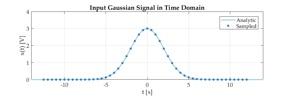
This code produces the following plots, which agree very nicely with the analytic expression above. Since $X(f)$ is real, we have $|X(f)| = X(f)$, and $\textrm{arg}(X) = 0$. (This is because the Gaussian in Eq. (1) is centered at $t = 0$. If the signal was shifted in time to $t=t_0$, this would introduce an addtional phase shift factor of $e^{-2\pi ift_0}$, and $\textrm{arg}(X)$ would be non-zero.)

The problem is that this code works, but I am not entirely sure exactly why it works!

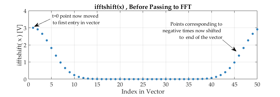
What confuses me is that I have had to use ifftshift(x) before passing my Gaussian to fft(), and fftshift(x) afterwards. I was careful to define my time vector in the code in such a way that the zero of time falls at the index $N/2+1 = 26$. This is because I know then that after ifftshift() the zero point will then be moved to the first entry in the vector (since I am using an even number of samples), as seen in the figure below:

Can someone explain why we have to do this. The most common justification I keep seeing is

"It's just because the FFT 'assumes' the time zero point is the first value in your vector!"

or

"It's just because of the periodicity of the DFT!"

Is there a nice way to see this explicitly in terms of the approximation to the continuous case, without anthropomorphizing the FFT algorithm and resorting to the above comments?

Ideally, I would like to see a mathematical proof which loosely says:

"if your time-domain signal is centered, the output of the FFT will only approximate the continous-time Fourier transform if the two halves of the vector are swapped, and you first move your zero to the front, and then move it back to the middle again afterwards. Otherwise the phase obtained will be wrong".

A proof of this nature would then justify the use of ifftshift() and fftshift() for me.

EDIT 1 ------ Without shifting, it doesn't work ------

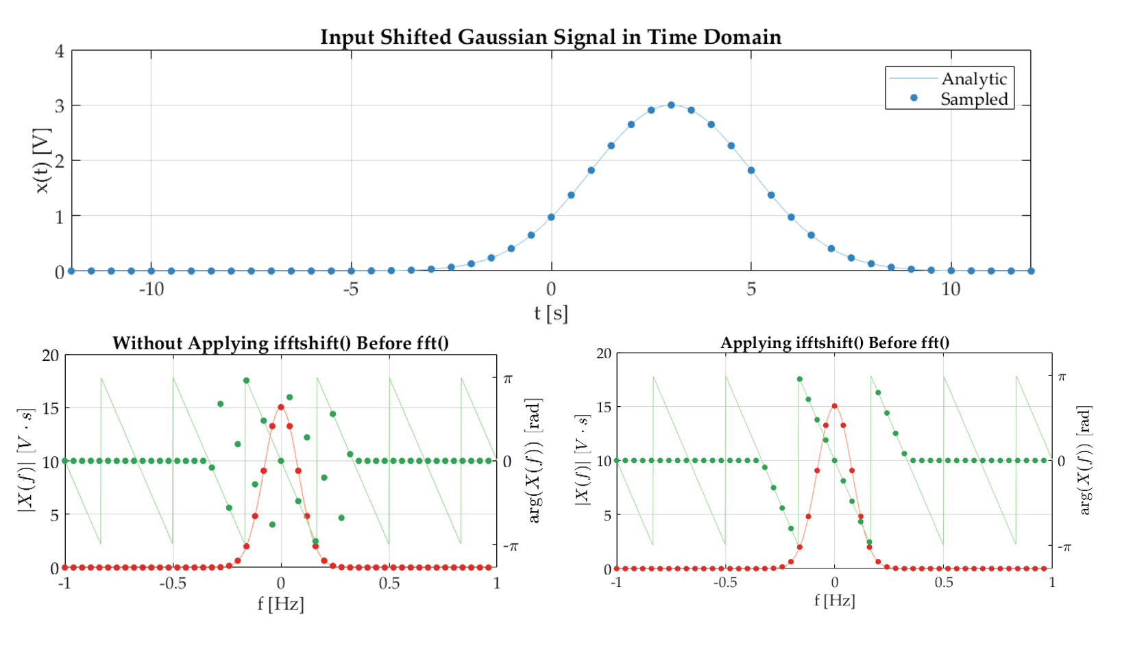
At the request of DSP Rookie, here is an example to show that if the input is actually a shifted Gaussian signal (centered at $t=3$), then the expected linear phase is only obtained if ifftshift() is applied to the signal before the fft() command, and fftshift() applied afterwards:

EDIT 2 ------ My own attempt ------

Here is my own attempt at what I am looking for, but I am struggling to finish it:

The goal is to calculate a numerical version of the Fourier transform: $$ X(f) = \int_{-\infty}^{+\infty} x(t) e^{-2\pi ift} \,\,\textrm{d}t $$ by using Matlab's fft() function.

Let's say I collect $N$ samples of $x(t)$ at specific times centered around zero-time with sampling period $T_s = 1/F_s$. The first sample is collected at time $t_1 = -T/2$, and the final sample collected at time $t_N=T/2 - T_s$, where $T = NT_s$. I can then define a sampled version of the signal which I will denote by $x[n]$ (I want to stick with Matlab's $n=1$ indexing convention for this exercise): $$ x[n] := x(t_n) = x\bigg( t=(n-1)\;T_s -\frac{T}{2}\bigg) \hspace{1cm} \textrm{for}\;\;\;\ n = 1,2,..., N $$ so that we have $$ \begin{align} x[1] &= x\bigg(t = -\frac{T}{2}\bigg)\\ x[2] &= x\bigg(t = -\frac{T}{2}+T_s\bigg)\\ &\vdots \\ x[N] &= x\bigg(t = \frac{T}{2}-T_s\bigg).\\ \end{align} $$ The sampled version of the signal would look like this:

I can write the CTFT formula as a Riemann sum, and insert this sampled signal into it (assuming I captured sufficiently the underlying signal) to obtain $$ \begin{align} X(f) &= \lim_{T_s\rightarrow0} \sum^{N}_{n=1} x[n] \exp \bigg( -2\pi i f \bigg[(n-1)\;T_s-\frac{T}{2}\bigg] \bigg)\cdot T_s\\ &\approx \sum^{N}_{n=1} x[n] \exp \bigg( -2\pi i f \bigg[(n-1)\;T_s-\frac{T}{2}\bigg] \bigg)\cdot T_s. \end{align} $$

Now in practice, the result is only going to give me values of $X(f)$ at certain frequencies $f_k$. Specifically, I am going to obtain $N$ values of the transform (neglecting zero-padding), centered around zero (because the CTFT that I am approximating runs from positive to negative), with the first frequency given by $f_1 = -F_s/2$ (the Nyquist). Each value in the vector will correspond to frequencies that increment by $\Delta f = F_s/N$, and so we can define a sampled verison of the transform by $$ X[k] := X(f_k) = X\bigg( f=(k-1)\;\Delta f -\frac{F_s}{2}\bigg) \hspace{1cm} \textrm{for}\;\;\;\ k = 1,2,..., N $$ so that we have $$ \begin{align} X[1] &= X\bigg(f = -\frac{F_s}{2}\bigg)\\ X[2] &= X\bigg(f = -\frac{F_s}{2}+\Delta f\bigg)\\ &\vdots \\ X[N] &= X\bigg(f = \frac{F_s}{2}-\Delta f\bigg).\\ \end{align} $$ Evaluating the approximation to the CTFT at these specific frequencies, I get $$ X[k] \approx \sum^{N}_{n=1} x[n] \exp \bigg( -2\pi i \bigg[(k-1)\;\Delta f-\frac{F_s}{2}\bigg] \bigg[(n-1)\;T_s-\frac{T}{2}\bigg] \bigg)\cdot T_s. \tag{4} $$ Now, this expression is clearly not that used by Matlab's fft() function, which is actually given here to be $$ Y[k] =\sum^{N}_{n=1} y[n] \exp \bigg( -2\pi i\; \frac{(n-1)(k-1)}{N} \bigg), \tag{5} $$ and so it is no surprise that simply passing the sampled signal straight to fft()*Ts without any modification does not give a way to approximate the CTFT of the orginal signal.

However, I do know that the command X[k] = fftshift(fft(ifftshift(x[n])))*Ts works, and produces the correct thing, because I have shown it in the graphs in the OP. So, this command must be equivalent to Eq. (4), but I am not sure how to mathematically prove it.

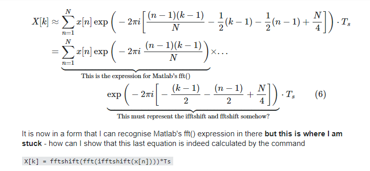
I can try to expand Eq. (4) as follows: $$ \begin{split} X[k] \approx &\sum^{N}_{n=1} x[n]\times ... & \\ &\exp \bigg( -2\pi i \bigg[(n-1)(k-1)\;\Delta f\; T_s - (k-1)\frac{T\Delta f}{2} -(n-1)\frac{T_sF_s}{2} + \frac{F_sT}{4}\bigg] \bigg)\cdot T_s \end{split} $$ and since $F_s = 1/T_s$, $F_sT=N$, and $\Delta f = F_s/N$, this simplifies to $$ \begin{split} X[k] &\approx \sum^{N}_{n=1} x[n] \exp \bigg( -2\pi i \bigg[\frac{(n-1)(k-1)}{N} - \frac{1}{2}(k-1) - \frac{1}{2}(n-1) + \frac{N}{4}\bigg] \bigg)\cdot T_s \\ &= \underbrace{\sum^{N}_{n=1} x[n] \exp \bigg( -2\pi i\; \frac{(n-1)(k-1)}{N} \bigg)}_{\text{This is the expression for Matlab's fft()}}\times... \\ &\hspace{3cm}\underbrace{\exp \bigg(-2\pi i\bigg[-\frac{(k-1)}{2} - \frac{(n-1)}{2} + \frac{N}{4}\bigg] \bigg)}_{\text{This must represent the ifftshift and fftshift somehow?}}\cdot T_s \hspace{1cm} (6) \end{split} $$

It is now in a form that I can recognise Matlab's fft() expression in there but this is where I am stuck - how can I show that this last equation is indeed calculated by the command

X[k] = fftshift(fft(ifftshift(x[n])))*Ts

I have a feeling that there might be a way to use the shift theorem to show that if you circularly shift the vectors through ifftshift and fftshift then you can cancel the extra phase factors, and the fft can be applied.

As a quick sanity check on Eq. (6) so far, I can verify it by manually evaluating the two things for a simple test vector of six numbers:

x = [1 2 3 4 5 6];
N = length(x);

%%% Calculate fft using MATLAB's fft (with ifftshift / fftshift)
X_WithShifts = fftshift(fft(ifftshift(x)));

%%% Calculate fft using MATLAB's fft (without ifftshift / fftshift)
X_WithoutShifts = fft(x);

%%% Calculate X using Eq. (6) formula (without using fft, ifftshift, or fftshift)
X_Manual = zeros(1,N);
for k = 1:N
   for n = 1:N
       X_Manual(k) = X_Manual(k) + x(n)*exp(-2*pi*1i*(n-1)*(k-1)/N)*...
           exp( -2*pi*1i*( -(k-1)/2 - (n-1)/2 + N/4 ) );
   end    
end

which gives the same results for each of the shifted versions, and does not work correctly if you don't use the shifting functions:

X_WithShifts = 
      [ (3+0i) (-3-1.73i) (3+5.20i) (21+0i) (3-5.20i) (-3+1.73i) ]

X_Manual = 
      [ (3+0i) (-3-1.73i) (3+5.20i) (21+0i) (3-5.20i) (-3+1.73i) ]

X_WithoutShifts = 
      [ (21+0i) (-3+5.20i) (-3+1.73i) (-3+0i) (-3-1.73i) (-3-5.20i) ] % WRONG

Answer 1

Problem Statement

Continuing with the OP's approach we will show how only in the case that N is an even number of samples, the following expression that was derived does match the operations noted with ifftshift and fftshift. We will also show the equivalent expression for the case that N is odd. As requested by the OP, this answer will be using MATLAB based indexing.

At the end we provide additional intuitive insight into what is occurring, which does not have anything to do with zero-phase.

---

Figure from OP copied below for reference:

---

Solution

In summary the result for fftshift(fft(ifftshift(x[n]))) is:

$$(-1)^{(k-1+\frac{N}{2})}\sum_{n=1}^N \bigg((-1)^{(n-1)}x[n]\bigg) W_N^{(n-1)(k-1)} \space\space\space \text{for N even}$$

$$j^N W_{4N}^{(k(2N+2)-3)} \sum_{n=1}^N \bigg(W_{2N}^{(N+1)n}x[n]\bigg) W_N^{(n-1)(k-1)}\space\space\space \text{for N odd}$$

See $\ref{8}$ and $\ref{9}$ below for further details on the notation used and how the case for $N$ even matches the OP's equation.

fft(ifftshift(x[n]))

The MATLAB command ifftshfit() undoes fftshift() and is a circular shift to the right of $\big\lfloor \frac{N+1}{2}\big\rfloor$ samples. Where $N$ is the number of samples in the DFT and $\lfloor \cdot \rfloor$ is the floor function.

$$\text{ifftshift}(x[n]) = x[n-m]\tag{1}\label{1}$$

With $m = \big\lfloor \frac{N+1}{2}\big\rfloor$

The DFT using MATLAB indexing is given as:

$$x[n] \leftrightarrow X[k]= \sum_{n=1}^Nx[n]W_N^{(n-1)(k-1)}\space\space\space\space n,k \in \{1,2...N\}\tag{2}\label{2}$$

With $W_N^n = e^{-j2\pi n/N}$

The effect of ifftshift() on the time domain samples is derived directly from the time shift property of the DFT given as follows and easily derived from $\ref{2}$:

$$x[n-m] \leftrightarrow W_N^{m(k-1)}X[k], \space\space\space\space n,k \in \{1,2...N\}\tag{3}\label{3}$$

Thus combining $\ref{1}$, $\ref{2}$, and $\ref{3}:$

$$\text{fft(ifftshift}(x[n])) = G[k] = W_N^{m(k-1)}\sum_{n=1}^N x[n]W_N^{(n-1)(k-1)}\tag{4}\label{4}$$

fftshift(G[k])

The MATLAB command fftshfit(x) is a circular shift to the left of $\lfloor \frac{N+1}{2}\rfloor$ samples:

$$\text{fftshift}(G[k]) = G[k+m]\tag{5}\label{5}$$

With $m$ as defined above for ifftshift(). (Equivalently, but not used here, this is a circular shift to the right of $\lfloor \frac{N-1}{2}\rfloor$ samples)

From $\ref{4}$ and $\ref{5}$

$$G[k+m] = W_N^{m(k-1+m)}\sum_{n=1}^N x[n]W_N^{(n-1)(k-1+m)} $$

$$= W_N^{m(k-1+m)}\sum_{n=1}^N x[n]W_N^{(n-1)(k-1)}W_N^{(n-1)m}$$

Resulting in the general expression for $N$ odd or even:

$$\text{fftshift(fft(ifftshift}(x[n]))) = W_N^{m(k-1+m)}\sum_{n=1}^N \bigg(W_N^{(n-1)m}x[n]\bigg) W_N^{(n-1)(k-1)} \tag{6}\label{6}$$

$$ G[k+m] = W_N^{m(k-1+m)}\text{FFT}\bigg\{W_N^{(n-1)m}x[n]\bigg\}$$

With $m = \big\lfloor \frac{N+1}{2}\big\rfloor$

Equivalence to OP's Equation (for N even)

For $N$ even, $m= N/2$ and $\ref{6}$ becomes:

$$G[k+N/2] = W_N^{\frac{N}{2}(k-1+\frac{N}{2})}\sum_{n=1}^N \bigg(W_N^{\frac{N}{2}(n-1)}x[n]\bigg) W_N^{(n-1)(k-1)} $$

Noting that $W_N^{N/2} = -1$, the above equation is:

$$G[k+N/2] = (-1)^{(k-1+\frac{N}{2})}\sum_{n=1}^N \bigg((-1)^{(n-1)}x[n]\bigg) W_N^{(n-1)(k-1)} \tag{7}\label{7} \space\space\space \text{for N even}$$

This is equivalent to the OP's equation:

$$X[k] =\sum_{n=1}^N x[n] \exp\bigg(-2\pi i \frac{(n-1)(k-1)}{N}\bigg)\times \ldots $$

$$\space\space\space \exp\bigg(-2\pi i \bigg[-\frac{(k-1)}{2}-\frac{(n-1)}{2}+\frac{N}{4}\bigg]\bigg) \tag{8}\label{8}$$

As follows:

Rearranging $\ref{7}$ to match $\ref{8}$:

$$G[k+m] = \sum_{n=1}^N x[n] W_N^{(n-1)(k-1)}(-1)^{(k-1+\frac{N}{2})} (-1)^{(n-1)}$$

$$= \sum_{n=1}^N x[n] W_N^{(n-1)(k-1)}(-1)^{(k-1)}(-1)^{\frac{N}{2}} (-1)^{(n-1)}$$

$$= \sum_{n=1}^N x[n] W_N^{(n-1)(k-1)}(-1)^{(k-1)}(-1)^{(n-1)}(-1)^{\frac{N}{2}}\tag{9}\label{9} $$

It should be clear that between $\ref{8}$ and $\ref{9}$ the first term that represents the DFT operation is equivalent:

$$\sum_{n=1}^N x[n] \exp\bigg(-2\pi i \frac{(n-1)(k-1)}{N}\bigg) =\sum_{n=1}^N x[n] W_N^{(n-1)(k-1)}$$

Given $W_N^n = \exp(-2\pi i \frac{n}{N})$

The second term in $\ref{8}$ is equivalent to $\ref{9}$ as follows:

$$\exp\bigg(-2\pi i \bigg[-\frac{(k-1)}{2}-\frac{(n-1)}{2}+\frac{N}{4}\bigg]\bigg)$$

$$= \exp\bigg(2\pi i\frac{(k-1)}{2}\bigg)\exp\bigg(2\pi i \frac{(n-1)}{2}\bigg)\exp\bigg(-2\pi i \frac{N}{4}\bigg)$$

$$= \exp\bigg(i \pi (k-1)\bigg)\exp\bigg(i \pi (n-1) \bigg)\exp\bigg(-i \pi \frac{N}{2}\bigg)$$

$$=(-1)^{(k-1)}(-1)^{(n-1)}(-1)^{\frac{N}{2}} \space\space\space \text{for N even}$$

For $N$ odd

For $N$ odd, $m= (N+1)/2$ and $\ref{6}$ becomes:

$$G[k+m] = W_N^{m(k-1+m)}\sum_{n=1}^N \bigg(W_N^{m(n-1)}x[n]\bigg) W_N^{(n-1)(k-1)} $$

$$ = W_N^{mk}W_N^{-m}W_N^{m^2}\sum_{n=1}^N \bigg(W_N^{mn}W_N^{-m}x[n]\bigg) W_N^{(n-1)(k-1)} $$

$W_N^{-m}$ can be pulled out of summation:

$$G[k+m] = W_N^{mk}W_N^{-2m}W_N^{m^2}\sum_{n=1}^N \bigg(W_N^{mn}x[n]\bigg) W_N^{(n-1)(k-1)}\tag{10}\label{10} $$

Reducing $W_N^{m^2}$ for $N$ odd:

$$W_N^{m^2} = W_{4N}^{(N^2+2N+1)}= W_4^NW_2^NW_{4N}^1$$

For $N$ odd this is:

$$W_N^{m^2} = W_4^NW_2^NW_{4N}^1 = (-j)^N(-1)W_{4N}^1= j^NW_{4N}^1$$

Substituting this back into $\ref{10}:$

$$G[k+m] = W_N^{mk}W_N^{-2m} j^NW_{4N}^1\sum_{n=1}^N \bigg(W_N^{mn}x[n]\bigg) W_N^{(n-1)(k-1)} $$

$$G[k+m] = j^N W_N^{m(k-2)+1/4} \sum_{n=1}^N \bigg(W_N^{mn}x[n]\bigg) W_N^{(n-1)(k-1)} $$

$$G\big[k+(N+1)/2\big] = j^N W_N^{\frac{N+1}{2}(k-2)+1/4} \sum_{n=1}^N \bigg(W_N^{\frac{N+1}{2}n}x[n]\bigg) W_N^{(n-1)(k-1)} $$

$$G\big[k+(N+1)/2\big] = j^N W_{2N}^{k(N+1)}W_N^{(-N-1)}W_{4N}^1 \sum_{n=1}^N \bigg(W_{2N}^{(N+1)n}x[n]\bigg) W_N^{(n-1)(k-1)} $$

$W_N^{(-N-1)} = W_N^{-1}$ so the above simplifies further to (for $N$ odd:

$$G\big[k+(N+1)/2\big] = j^N W_{4N}^{(k(2N+2)-3)} \sum_{n=1}^N \bigg(W_{2N}^{(N+1)n}x[n]\bigg) W_N^{(n-1)(k-1)}\tag{11}\label{11} $$

Exact CTFT Result from DFT

The above proved the equivalence of the OP's equation as further requested as well as what the relationship would be for $N$ odd. Below are further details going back to the more general question of the OP:

The OP wants to prove why the following MATLAB command "matches the samples of the CTFT":

X = fftshift(fft(ifftshift(x)));

While the following does not:

X = fft(x);

Caveats

For a Discrete Fourier Transform (DFT) to match samples of the Continuous-Time Fourier Transform (CTFT), the signal unless sampled (and therefore periodic in frequency) must have no spectral occupancy beyond the sampling rate, or will otherwise deviate due to the effect of the aliasing from those higher frequencies. Further the CTFT is a continuous time integration involving the function x(t), and any summation expressions on samples of x(t) are numerical approximations (such as Forward Euler, Backward Euler, Tustin, etc) whose results improve as the sampling rate is increased but (to my understanding) none can provide an exact match, so similarly an exact match to the underlying CTFT cannot be derived from the DFT, although can be closely approximated for sufficiently large sampling and no aliasing (this last sentence must be confirmed).

Under the condition of no aliasing, with proper scaling the Discrete Time Fourier Transform (DTFT) will be closely matched to the CTFT over the CTFT frequency range $f \in [-f_s/2, f_s/2)$ (first Nyquist zone) where $f_s$ is the sampling rate, since both are continuous functions.

For causal time limited sequences, with proper scaling, the The DFT as computed by fft() will be identical to samples of the DTFT over the DTFT frequency range $f \in [0, f_s)$, as beyond the first Nyquist zone, the DTFT can be assumed to be periodic in frequency with a period of $f_s$ with relation to the CTFT.

Further, by definition the MATLAB time index $n=1$ (using MATLAB indexing per the OP's request) corresponds to $t=0$ in the CTFT time waveform $x[t]$. This is not "assumed" but clearly defined. This is easily confirmed by observing the phase response versus frequency for the two sequences [1 0] and [0 1], where we see that fff([1 0] has no phase shift consistent with an impulse at $t=0$. Similarly, the MATLAB frequency index $k=1$ corresponds to $f=0$ in the CTFT frequency waveform $X(f)$.

Given this, the MATLAB fft() function already matches samples of the CTFT for causal time domain waveforms! The OP desires to modify the result of the MATLAB fft() function so that other time and frequency indexing can be used. Such alternate indexing must be defined as to where the new assumed index positions will be corresponding to $t=0$ and $f=0$. Since the DFT is circular in both time and frequency (periodic related to the CTFT where the frequency axis extends to $\pm \infty$), this desired modification is accomplished by circularly shifting the time and frequency indexes.

If the first MATLAB expression above fftshift(fft(ifftshift(x))) "matches a CTFT" according to the OP, then this dictates what the OP's assumption is for the MATLAB index positions for the time and frequency arrays that correspond to where $t=0$ and $f=0$ in the DTFT time and frequency arrays as summarized below:

Desired MATLAB index to represent $t=0$ in the DTFT time array:

$n_{t=0}=\lfloor N/2\rfloor+1 \tag{12}\label{12}$

Desired MATLAB index to represent $f=0$ in the DTFT frequency array:

$k_{f=0}=\lceil N/2\rceil+1 \tag{13}\label{13}$

Where $\lfloor \cdot \rfloor$ represents the floor function and $\lceil \cdot \rceil$ represents the ceiling function.

To stress, these choices are completely arbitrary (see Side Note below) and the main objective here is to quantify with equations how to predict the CTFT result from the MATLAB fft() result given alternate definitions for where $t=0$ and $f=0$ would be in the DTFT instead of the default of $n=1$ and $k=1$, in this case per the time and frequency shifts given by $\ref{12}$ and $\ref{13}.

It is directly clear that the above two operations are exactly what is performed by ifftshift() and fftshift() respectively.

Side Note: Another (better?) shifting approach to consider:

The OP selected alternative indexing for the DFT as the intention was to show the results for time and frequency sequences that have $t=0$ and $f=0$ centered in the sequence. This is a matter of personal selection no different than deciding what range is desired for the x-axis on a plot since the DFT repeats over any range selected. An alternate approach to accomplish this follows such that the first sample is always centered, as the choice given by the OP results in positioning $t=0$ and $f=0$ with a one sample offset when the number of samples $N$ is even. To have a middle sample represent $t=0$ and $f=0$ requires an odd number of samples. A mapping that will keep the center sample at $t=0$ and $f=0$ while not changing DFT values (except for the middle sample) can be accomplished by doing the following to create an odd sequence for the case that $N$ is even. This is presented using the samples with MATLAB Indexing from $1:N$, with $f[n]$ representing the $N$ time samples and $F[k]$ the $N$ frequency samples:

Place the first sample $f[1], F[1]$ to be in the middle of the sequence.

Place the next $N/2-1$ samples after the first sample

Divide the sample at index $N/2$ in half, and use that as the next sample.

Place the other half of the sample at index $N/2$ to be at the start of the sequence.

Place the remaining samples between the start and middle of the sequence.

For example an even sequence: [9 2 5 3 1 12] would map to [1.5 1 12 9 2 5 1.5]

Where an odd sequence: [9 2 5 3 1] would map to [3 1 9 2 5]

---

Intuitive Explanation

This has nothing to do with zero-phase or linear phase as other responses have indicated, as the sequence given by $x(t)$ can be a complex sequence and therefore may have non-linear phase before or after the fftshift() commands. What this has everything to do with is that the Discrete Fourier Transform (DFT) as defined (not assumed) assumes $t=0$ as the first sample, while the OP is comparing its use to non-causal waveforms where $t=0$ at or near the center of the sequence. Similarly the OP would like to present the frequency result with $f=0$ at or near the center of the sequence.

The time index must be defined if used any differently from the DFT definition. The DFT will match the DTFT (as samples of the CTFT) with no modification other than scaling when we assume the waveform for the DTFT is causal and starts at $t=0$ in the CTFT (with the restriction that the waveform cannot have spectral content above the sampling rate), and when we assume the samples from the fft() result start at $f=0$ in the CTFT. Any other changes to the index positions related to the DTFT and CTFT $t=0$ and $f=0$ positions will require shifting the sequences accordingly in time and frequency. Therefore it is useful to summarize for reference the Fourier Transform time and frequency shift properties.

Summary of Fourier Time and Frequency Shift Properties:

CTFT Shift Properties ($t,T,\omega, \omega_o \in\mathbb{R}$)

$${x(t-T)} \leftrightarrow e^{-\omega T}X_C(\omega) \tag{14} \label{14}$$

$$e^{\omega_o t}x(t) \leftrightarrow X_C(\omega-\omega_o) \tag{15} \label{15}$$

DTFT Shift Properties ($n,m\in\mathbb{Z}$, $\omega, \omega_o\in[-\pi, \pi)$)

$$x[n-m] \leftrightarrow e^{-\omega m}X_{2\pi}(\omega) \tag{16} \label{16}$$

$$e^{\omega_o n}x[n] \leftrightarrow X_{2\pi}(\omega-\omega_o) \tag{17} \label{17}$$

DFT Shift Properties ($n,m,k,\ell\in\{1\ldots N\}$)

$$f[n-m] \leftrightarrow W_N^{m(k-1)}F[k], \tag{18} \label{18}$$ $$W_N^{-\ell (n-1)}x[n] \leftrightarrow F[k-\ell], \tag{19} \label{19}$$

Where:
$W_N^{m} = e^{-j2\pi m/N}$ (The roots of unity)
$\mathbb{Z}$ is the set of all integers, whether positive, negative or zero: [..., −2, −1, 0, 1, 2, ...]
$\mathbb{R}$ is the set of all reals

The ifftshift() and fftshift() commands are simply moving the reference index for $t=0$ and $f=0$ to be at the alternate positions given in $\ref{12}$ and $\ref{13}$. Similarly the time index shift could be done directly on the fft() result $F[k]$ using $\ref{18}$ and the frequency index shift could be done directly on the time samples $x[n]$ using $\ref{19}$.

Answer 2

Answer: ifftshift() is required to make the sampled Gaussian symmetric modulo N in discrete time-domain. In continuous time it is already symmetric around t=0, which is the only requirement for continuous-time fourier transform of a real valued function to be real valued zero-phase. But When you approximate the gaussian in discrete time by starting the pulse sampling at some negative T to positive T, like $t=-(T/2):Ts:(T/2 -Ts)$, then the gaussian is doesnot remain symmetric modulo N. "ifftshift()" does exactly that.

For, DFT/FFT to have zero phase, DFT should be real. Hence, $X[k] = X^*[k]$, to achieve this, the time-domain real valued sequences should satisfy the following:$$x[n] = x[(N-n)\mod \ N]$$This means that except x[n] at n=0, all of the other samples of $x[n]$ should be mirror image across $N/2$-point. "ifftShift()" operation in MATLAB does exactly that. If you see your ifftshifted sampled plot of gaussian, notice that $x[0]$ is Gaussian pulse value at $t=0$, but all of the N/2 values corresponding to $t=-(T/2):-Ts$ are placed now as mirroe image of values corresponding to $t=Ts:(T/2)-Ts$. That is why use of ifftshift makes phase response zero-phase.

Derivation of the above property: $$X^*[k] = (\sum^{N-1}_{n=0}x[n].e^{-j\frac{2\pi}{N}nk})^* = \sum^{N-1}_{n=0}x^*[n].e^{j\frac{2\pi}{N}nk}$$Since $x[n]$'s are real valued hence $x^*[n]=x[n]$, so, $$X^*[k] = \sum^{N-1}_{n=0}x[n].e^{j\frac{2\pi}{N}nk}$$Equating this to $X[k]$ will give us: $$x[n] = x[(N-n)], \forall n=1,2,3,4,...,\frac{N}{2}$$ This means that for DFT of a real valued sequence to be real-valued, the $x[n]$ should be symmetric modulo N.

-------------- EDIT ----------------

Adding the DFT analysis changing the sum limits from $\{0,...,(N-1)\}$ to $\{-N/2,...,N/2-1\}$.

$$X_s[k] = \sum^{N/2 - 1}_{n=-N/2} x[n]e^{-j2\pi /N nk}$$Substitute $m=n+N/2$ $$X_s[k] = \sum^{N - 1}_{m=0} x[m-\frac{N}{2}]e^{-j2\pi /N (m-\frac{N}{2})k}$$ $$X_s[k] = \sum^{N - 1}_{m=0} x[m-\frac{N}{2}]e^{-j\frac{2\pi}{N}mk}.e^{j\frac{2\pi}{N} \frac{N}{2} k}$$ $$ = (-1)^k \sum^{N - 1}_{m=0} x[m-\frac{N}{2}]e^{-j\frac{2\pi}{N}mk}$$And, as i have said in the comment, $x[-N/2] = x(-T/2)$, $x[-N/2 + 1] = x(-T/2 + Ts)$, .... $x[0] = x(0)$, ....., $x[N/2 - 1] = x(T/2 - Ts)$. Substitute them and figure out that the new DFT $X_s[k]$ is also real valued because, if the the time domain function $x(t)$ was real valued and symmetric about $t=0$, then $X_s[k] = X_s^*[k]$. And, with this DFT definition you do not have to use ifftshift(). You can write the above $X_s[k]$ in MATLAB and then verify the result.

Answer 3

The FFT is just an fast algorithm to implement the Discrete Fourier Transform (DFT) which is defined as

$$ X(k)= \sum_{n=0}^{N-1}x(n) \cdot e^{-j2 \pi \frac{n \cdot k}{N} } $$

Both the time and frequency domain signals are discrete. This implies they are periodic in the other domain: when you discretize a signal in one domain you force it to be periodic in the other.

The periodicity also means that there is really no start or end point. You can actually start summing at any point in time and you will get the same result. you could sum from -N/2 to N/2-1 or from N/2+1 to N/2 and it would still all work.

At this point it becomes more a less a question of convention. There are cases where summing from 0 to N-1 is more intuitive and sometime -N/2 to N/2-1 is more intuitive. For most time domain signals, the first one makes more sense and it's also the cleanest mathematically so that's one of choice at the moment.

Answer 4

Note that the phase zero reference point of an FT is where the cosine or real component of all the exponential basis vectors is 1.0, and where the sine or imaginary component is not only zero, but has a 1st derivative of 1.0. This only occurs in a DFT or FFT at sample 0 of all basis vectors from 0 to N-1.

At the center (or N/2 of N even), the 1st derivative of the sine or imaginary component flips from -1.0 to 1.0 between basis vectors (crosses zero in the opposite directions for odd periodic and even periodic basis exponentials). So that does not meet the criteria for being the phase zero reference of an FT.

Thus the need for an fftshift (for even N).

This works because all the DFT basis vectors are circular, thus any rotation of the input data just results in a shift to needed phase reference.

As for clipping the limits from -N/2 to N/2 instead of -inf to inf: if the area under the curve from N/2 to inf is on the order of or less than the numerical noise (quantization, rounding, etc.) then you might not even notice the difference after printing or plotting to some readable number of significant digits.