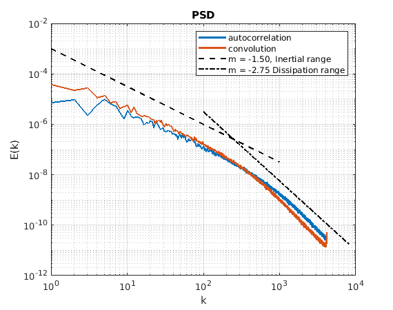
I have a 1D fractional Brownian motion (fBm) signal, $u(x)$, of size $N$, generated through a random number generator with a gaussian mean, $\mu=0$, and standard deviation, $\sigma=\sqrt{N}$. I want to find the power spectral density (PSD) of said signal. Signal data, MATLAB-R2018a code, and citation is included in the Github repository (https://github.com/dustinma324/Buruglence) .
From "Numerical Recipes" by Press 2007, $$ Corr(g,h)_{j} = G_{k}H_{k}^* $$ where $G_{k}$ and $H_{k}$ are the discrete Fourier transforms (DFT) of $g_{j}$ and $h_{j}$, and the asterisk represents the complex conjugate. Normalizing the above equation by $N^2$ returns the PSD.
I am having trouble understanding the difference between the order of performing DFT. I have two road maps in mind to get the PSD. The first being,
$$ PSD = fft\Big(u(x)\Big) \cdot fft\Big(u(x)\Big)^{*} $$
where the PSD is found through breaking up the auto-correlation function into the product of the Fourier transform and the complex conjugate of the Fourier transform (convolution) of the two signals. The second,
$$ R_{11}(r) = u(x)*u(-x)$$ $$ PSD = \bigg|fft\Big(R_{11}(r=0) \Big)\bigg| $$
where the PSD is found by finding the auto-correlation function of the signal first, then taking the magnitude of the Fourier transform of the auto-correlation function.
The dark blue line is the second method, and red is the first. By taking the $FFT$ of the auto-correlation function, the general shape is captured, but the latter method shows small amounts of energy accumulation at the higher frequencies. This violates the Schwartz inequality, since the inner product of to vectors cannot be larger than the product of their magnitudes.
Is there a specific mathematical reason as to why the latter method appears to carry more energy at the higher frequencies?
Here's my MATLAB code below for the two different methods.
Method 1 (Convolution)
n = length(x); %Nx
pwr = [];
meanU = mean(u(:,tavg_start:end),2);
for i = tavg_start:1:nt
   U_fft = fft(u(:,i)-meanU,n)/n;
   pwr = [pwr U_fft.*conj(U_fft)];
end
meanpwR = mean(pwr,2);
Method 2 (Auto-correlation function)
pwR = [];
n = length(x);
meanU = mean(u(:,tavg_start:end),2);
for i = tavg_start:step:nt
    U11 = double(u(:,i)-meanU);
    Ucorr = xcorr(U11); % Output will be 2*length(Ucorr)
    N = 2^nextpow2(length(Ucorr));
    R_fft = fft(Ucorr,N)/(N^2);
    pwR = [pwR abs(R_fft)];
end
meanpwR = mean(pwR,2);
I have not been able to find anything that explains my particular question. Any inputs/suggestions/discussions would be greatly appreciated.
UPDATE Feb 4th, 2020
Auto-correlation function is analogous to a low-pass filter, meaning low frequencies are getting through, and high frequencies are attenuated out (gradual loss) at a certain cutoff frequency. The attenuated frequencies (unresolved energy) is being aliased into lower level frequencies when performing the Fourier transform of the ACF, resulting in the slight increase.
A transition band was described in this link (https://www.ni.com/en-us/innovations/white-papers/18/anti-aliasing-filters-and-their-usage-explained.html). I believe for me this band ranged from $k = N/2$, Nyquist frequency, to $k=2N/3$, where Basu dealiased the same signal using the 3/2 rule in the Fourier domain. This band is said to cause aliasing in the signal, thus showing up in my graph above.
Technically both methods shows some form of aliasing. So are there different kinds of aliasing? One is observed to aliased over a range of wavenumbers, while the other shows a spike.
Thanks,
Dustin

