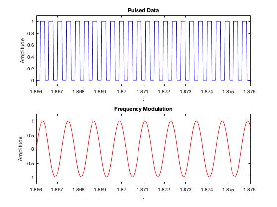
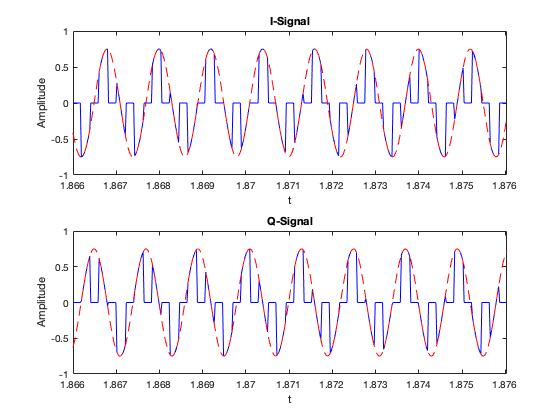
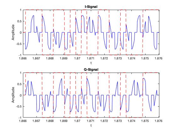
The IQ data looks like a sinusoidal modulated pulse train with binary phase shift keying (BPSK) superimposed. The BPSK symbol rate appears to be at the same rate as the pulse repetition frequency (PRF).
I was bored, so I went ahead and modeled the data in MATLAB.
clear; clc;

% Measured quantities from IQ data
pw = 2.1771e-4;         % Pulse Width
pri = 4.1123e-4;        % Pulse Repetition Interval
ts = 2.419e-5;          % Sampling Interval
period = 0.0012;        % Modulation Period
npulses = 24;           % Pulses in IQ plot
t_start = 1.8660;       % Plot start time

% Derived Quantities
prf = 1/pri;            % Pulse Repetition Frequency
fs = 1/ts;              % Sampling Rate
f = 1/period;           % Modulation Frequency

% Generate pulsed data
waveform = phased.RectangularWaveform('SampleRate',fs,'PRF',prf,...
    'PulseWidth',pw,'OutputFormat','Pulses','NumPulses',npulses);

pulses = waveform();

% Prepend data with zeros to match IQ plot
pulses = [zeros(fix((pri-pw)/ts),1); pulses].';

t = (0:length(pulses)-1)*ts;
t = t_start + t;

modulation = sin(2*pi*f*t);

figure(1)
subplot(2,1,1)
plot(t,pulses,'b'); title('Pulsed Data')
xlabel('t'); ylabel('Amplitude');
ylim([-0.1 1.1])
xlim([t(1) t(end)])

subplot(2,1,2)
plot(t,modulation,'r'); title('Frequency Modulation')
xlabel('t'); ylabel('Amplitude');
ylim([-1.25 1.25])
xlim([t(1) t(end)])

% Frequency Shifted Baseband Data
initial_phase = 3*pi/16;  % Used to match IQ plot
amp = 0.75;
I_mod = -amp*sin(2*pi*f*t + initial_phase);
Q_mod = -amp*cos(2*pi*f*t + initial_phase);

% Modulate the pulsed data
I_data = I_mod.*pulses;
Q_data = Q_mod.*pulses;

figure(2)
subplot(2,1,1)
plot(t,I_data,'b'); title('I-Signal');
hold on;
plot(t,I_mod,'r--');
xlabel('t'); ylabel('Amplitude');
ylim([-1.0 1.0])
xlim([t(1) t(end)])

subplot(2,1,2)
plot(t,Q_data,'b'); title('Q-Signal');
xlabel('t'); ylabel('Amplitude');
hold on;
plot(t,Q_mod,'r--');
ylim([-1.0 1.0])
xlim([t(1) t(end)])

% Phase Modulation
phase_code = [1 1 1 -1 -1 1 1 -1 1 -1 1 -1 -1 1 1 -1 -1 1 -1 -1 -1 1 1 1];
phase_chip = ones(1,pri/ts);

phase_mod = kron(phase_code,phase_chip);

% Prepend the data to match IQ plot
phase_mod = [zeros(1,fix((pri-pw)/ts)) phase_mod];

% Modulate the pulses data
I_phase = I_data.*phase_mod;
Q_phase = Q_data.*phase_mod;

figure(3)
subplot(2,1,1)
plot(t,I_phase,'b'); title('I-Signal');
hold on
plot(t,phase_mod,'r--')
xlabel('t'); ylabel('Amplitude');
ylim([-1.0 1.0])
xlim([t(1) t(end)])

subplot(2,1,2)
plot(t,Q_phase,'b'); title('Q-Signal');
hold on
plot(t,phase_mod,'r--')
xlabel('t'); ylabel('Amplitude');
ylim([-1.0 1.0])
xlim([t(1) t(end)])

In the figure above, you can see where the 180 degree phase shifts occur. I also found the ratio of the symbol rate (PRF) to modulation frequency (f) to be 2.91.
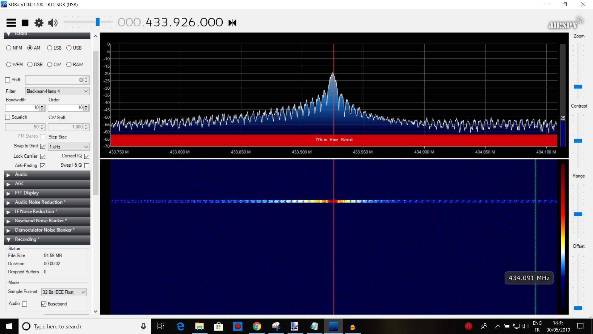 I can see there is only one peak with progressively decreasing peaks, so I assume this is AM. Then I set the bandwidth to the width of the central lobe. I finally made a recording of the "Audio" and opened the WAV into Audacity but I could not make sense of the sines (I was expecting a digital stream, since the modulation was specified) so here is the I/Q data instead.
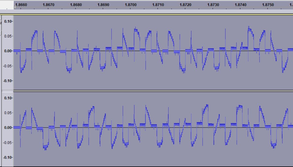 This is an extract of the body of this waveform:
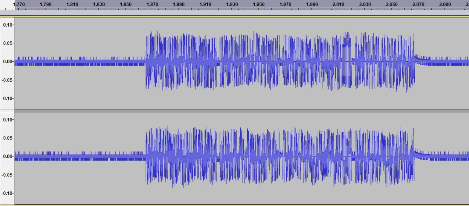 I have also installed DSD+ and the SDR# plugin as well as the virtual cable between the two, but after setting up SDR# the waveform does not budge so nothing comes up.

