Convolution with an impulse response does not give the same result as the frequency response

Question

Context

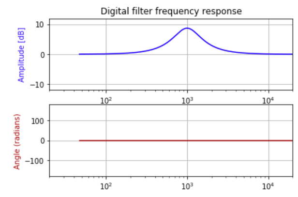
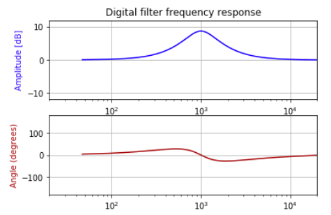
I am trying to design a linear-phase FIR filter with the following frequency and phase responses:

Designing the filter

Given its characteristics (peak filter at 1kHz with 9dB gain and Q=7), I got the following IIR biquad coefficients:

$$b_0 = 1.0889938082113808$$ $$b_1 = -1.8806408829603927$$ $$b_2 = 0.80787505079350063$$ $$a_0 = 1$$ $$a_1 = -1.8806408829603927$$ $$a_2 = 0.89686885900488144]$$

I then computed the impulse response of that biquad filter and truncated it to 1024 taps. I got the following filter:

To make the phase of my FIR filter linear, I applied an FFT on its impulse response, I put the imaginary part to 0 and came back to time domain by doing an inverse FFT.

The final taps I got can be found there.

The problem

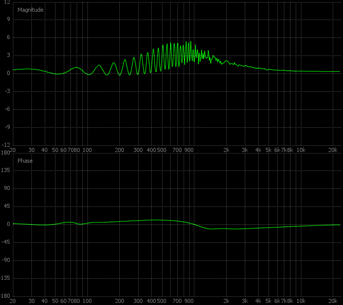
Now, when I plot the frequency/phase responses of this filter using Numpy/Scipy or Matlab, I get exactly the same plot as the one of my expected filter (see figure 1). But, when I apply this filter on a pink noise signal by convolution and measure the transfer function, I get this instead:

I am pretty lost here, I would assume that convolving my noise signal with my filter and measuring the transfer function would give me the same curve as the one I computed theoritically but it seems not to be the case (that is, in my mind, the definition of what convolution does).

Some additional information:

1. I have verified that the problem does not come from my implementation of the convolution operation, by testing with many different implementations; if you still believe the problem come from there, you can try yourself with the taps I provided.
2. I trust the software I used to measure the transfer function depicted in the last plot, and anyway I could hear that the transfer function is not the one I expect.

3. To plot the transfer functions from Python, I used the following code:

   import matplotlib.pyplot as plt
   import numpy as np
   from scipy import signal
   
   def plot_transfer_function(b, a=1):
       """Plot the frequency and phase response of a digital filter."""
       w, h = signal.freqz(b, a)
   
       fig = plt.figure()
       plt.title('Digital filter frequency response')
   
       # Frequency response
       ax1 = fig.add_subplot(211)
       plt.semilogx((w * SAMPLING_RATE) / (2 * np.pi), 20 * np.log10(abs(h)), 'b')
       # Make the plot pretty
       plt.ylabel('Amplitude [dB]', color='b')
       plt.xlabel('Frequency [Hz]')
       plt.axis([20, 20000, -12, 12])
       plt.grid()  # show the grid
   
       # Phase response
       ax2 = fig.add_subplot(212)
   
       angles = np.unwrap(np.angle(h))
       plt.semilogx((w * SAMPLING_RATE) / (2 * np.pi), np.degrees(angles), '#aa0000')
       # Make the plot pretty
       plt.ylabel('Angle (degrees)', color='#aa0000')
       plt.axis([20, 20000, -180, 180])
       plt.grid()
   
       fig.axes[0].set_axis_off()  # disable main figure axis
   
       plt.show()
   
   plot_transfer_function(TAPS)  # "TAPS" is an array containing the 1024 taps
   

So, what is wrong with my reasoning here? Why do I not measure the same frequency/phase response when calculating it and when measuring it after a convolution?

---

Additional question: for my FIR filter to have linear phase, I thought it should be symmetric (or anti-symmetric). Well, when I plot my 1024 taps, they appear to be pretty symmetric, excepted the first which does not have its equivalent at the end of the impulse response. Why is it so?

Answer 1

Explicitly making the imaginary part of your FFT coefficients 0 will change your magnitude response.

It is very clear if you consider this: $$ X_k = a_k + jb_k\\ |X_k| = \sqrt{a_k^2 + b_k^2} $$ Now, you're explicitly setting new coefficients to be $X'_k = a_k$, and hence $|X'_k| = |a_k|$. Taking the IFFT of your new frequency response will obviously not be the same as the impulse response you expect.

If instead you made $X'_k = |X_k|$ and then performed an IFFT, you would get your expected filter taps. This is because your magnitude response is enforced to be the same and your phase is enforced to be zero.

Answer 2

Setting the imaginary components of the FFT of a FIR filter to zero is not the way to make a linear phase filter with the same magnitude response as the FIR filter.

Added: Try using the magnitude of the complex valued FFT result instead.