Butterworth band pass filter

Question

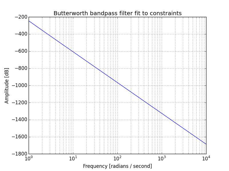
I am trying to build a Butterworth bandpass filter. My intent is to have a pass band between $250\textrm{ Hz}$ and $1000\textrm{ Hz}$. However the plot doesn't look right, as can be seen from the following graph:

Below is my code:

import scipy
import numpy as np
from scipy import signal
import matplotlib.pyplot as plt

#apply bandpass filter
fs = 8000
fso2 = fs/2.
N,Wn = scipy.signal.buttord(wp=[250./fso2,1000./fso2], ws=[200./fso2,1200./fso2],
   gpass=0.1, gstop=30.0)

b, a = signal.butter(N, Wn, 'band', True)
w, h = signal.freqs(b, a, np.logspace(0, 4, 500))
plt.semilogx(w, 20 * np.log10(abs(h)))
plt.title('Butterworth bandpass filter fit to constraints')
plt.xlabel('Frequency [radians / second]')
plt.ylabel('Amplitude [dB]')
plt.grid(which='both', axis='both')
plt.show()

Answer 1

You need to specify your filter design specifications parameters consistently for either an analog or a digital filter. With your posted code, the butterord computes the required order for a digital filter with cutoff frequencies near 1 (which would make sense as Nyquist-normalized cutoff frequencies, but not so much in Hz), then uses those directly to obtain analog filter coefficients.

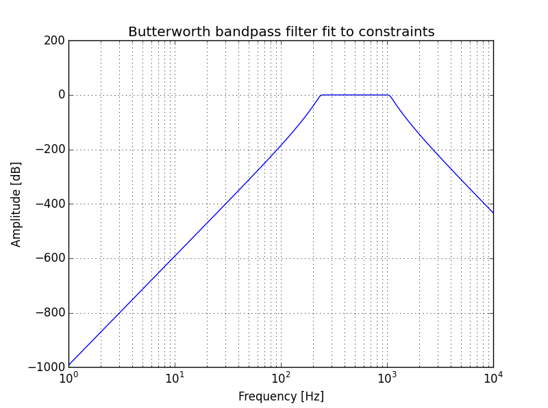
Depending on your application, you can either design an analog filter with

N,Wn = scipy.signal.buttord(wp=[250.,1000.], ws=[200.,1200.],
   gpass=0.1, gstop=30.0, analog=True)
b, a = signal.butter(N, Wn, 'band', True)
w, h = signal.freqs(b, a, np.logspace(0, 4, 500))

which should then produce a graph which looks like:

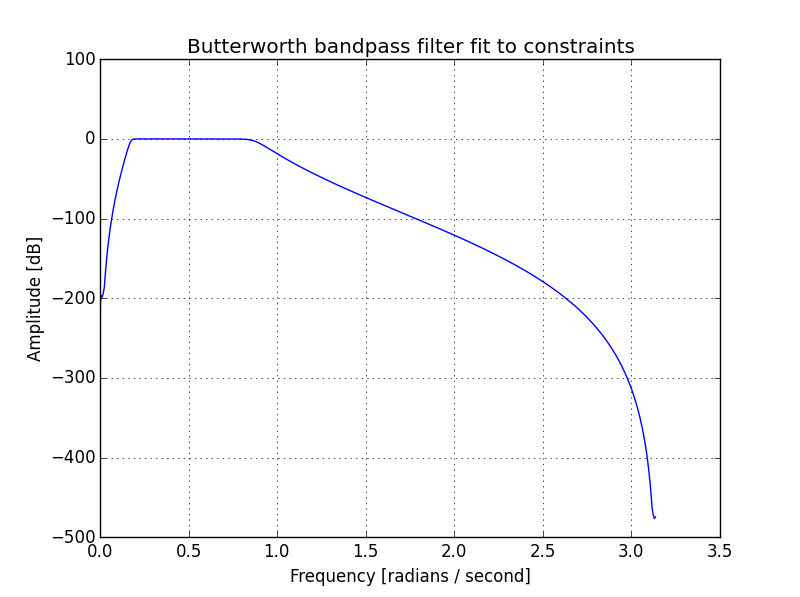
Alternatively you could design a digital filter with

N,Wn = scipy.signal.buttord(wp=[250./fso2,1000./fso2], ws=[200./fso2,1200./fso2],
   gpass=0.1, gstop=10.0, analog=False)
b, a = signal.butter(N, Wn, 'band', False)
w, h = signal.freqz(b, a)

Note however that the original specifications for a digital filter result in an 18^th-order filter which may start to show some artifacts due to numerical accuracy. As such I've reduced slightly the gstop parameter to produce the following graph: