0
$\begingroup$

I am relatively inexperienced with respect to lowpass filters, but I am trying to replicate parts of this paper, which deals with the processing of 3D accelerometer and 3D gyroscope data, both from the same IMU. The data has been collected at 50Hz (see p.5). A little bit later on p.5 it says that the data

is smoothed with a Butterworth low-pass filter (-60db at 20Hz).

No information about the order is given.

I code in Python so I am using Scipy's (v1.1.0) signal.butter (documentation), which requires to set

  • order N
  • critical frequency Wn
  • analog or digital
  • type of output

I found in the answer to this post, that I should use analog=False since my data has most likely been sampled regularly, which is what I expect from an IMU. However, I am very uncertain what is meant by

-60db at 20Hz.

I assume the cutoff frequency fc to be 20Hz, because the sampling frequency fs is stated in the paper as 50Hz.

Providing a time series snippet (only 1D for simplicity) for reproduction, this leaves me with this code:

import matplotlib.pyplot as plt
from scipy import signal

data = [-1.0436051383321092, -1.0505922388438984, -1.054092916480489, -1.0594615377516436, -1.0528397348040082, -1.0265495609876023, -1.0030861099986423, -1.0092599433155374, -1.0249089063356631, -1.0140387164631766, -1.0056669772119422, -1.0036560772602825, -0.9996307058908602, -0.9938863276199182, -0.9736733666046808, -0.9614502798619106, -0.9721199408045632, -0.9823970563524684, -0.9922003136484135, -1.0105170817955498, -1.0230552960961752, -1.0126115584815136, -0.9965836060956084, -0.9722516530084516, -0.9739932157698056, -0.9672539544164604]

fc = 20  # cutoff frequency ?
fs = 50  # sampling frequency

sos = butter(N=2, Wn=20/(50/2), btype='lowpass', analog=False, output='sos')  # not sure about the order N
filtered_data = sosfilt(sos, data)

plt.plot(data)
plt.plot(filtered_data)
plt.show()

Now I have three questions, which aim at finding out whether I replicated the filter correctly:

  1. Is there a way to infer N form the information given by the paper? I know that there is scipy.signal.buttord but I am afraid that the paper does not provide sufficient information to assign all required arguments.

  2. What is meant by "-60db at 20Hz"?

  3. Is it correct to use output='sos' and, subsequently, scipy.signal.sosfilt for smoothing this kind of data (6-dimensional IMU)?

$\endgroup$
1
  • $\begingroup$ It might mean "-60 dB/decade with a cutoff of 20 Hz"? The paper also mentions "First, an elliptical bandpass filter (0.15Hz – 11Hz) ". You'd have to look at the typical signal frequencies to figure out what is kept and what is filtered. You can reproduce the results without reproducing the exact filter. $\endgroup$
    – endolith
    Commented Jun 2 at 21:29

2 Answers 2

0
$\begingroup$

Is there a way to infer N form the information given by the paper? I know that there is scipy.signal.buttord but I am afraid that the paper does not provide sufficient information to assign all required arguments.

No there is not as the order and cutoff frequency is a trade as the complexity of a filter is inversely proportional to the steepness of the transition band. I'll demonstrate this below along with provide a filter solution:

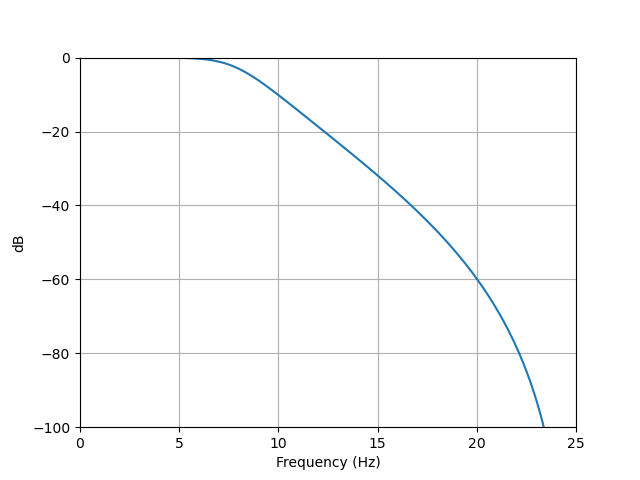
Below shows the Butterworth implementation with 60 dB attenuation at 20 Hz. This was done with a 4th order filter, and in order to reach 60 dB the cutoff frequency was set to 8 Hz:

fs = 50
coeff= sig.butter(4, Wn=8, fs=fs)
f, h= sig.freqz(*coeff, worN=2**18, fs=fs)
plt.figure()
plt.plot(f, 20*np.log10(np.abs(h)))
plt.grid()
plt.axis([0, 25, -100, 0])

frequency response

If a higher cutoff frequency is desired, the order would need to be increased to still achieve 60 dB attenuation at 60 Hz.

What is meant by "-60db at 20Hz"?

This is a specification on the attenuation the filter is to provide at a 20 Hz frequency (see my plot above). To achieve this, the cutoff frequency of the lowpass filter must be something below this value. The shorter the distance to the cutoff frequency, the higher the order of the filter that will be needed to achieve this attenuation.

Is it correct to use output='sos' and, subsequently, scipy.signal.sosfilt for smoothing this kind of data (6-dimensional IMU)?
If you were to implement this filter (rather than simulate the results), the the 'sos' form (second-order sections) is the go-to form for filter implementation. This factors a higher order filter into the cascade of smaller second order sections, which results in much more stable structures for implementation (and for that reason is also preferred when simulating very high order filters). For the 4th order example as I provided here, you should get the exact same results if you use 'ba' (as I did) or 'sos' (either can be used) for purposes of simulation.

$\endgroup$
0
$\begingroup$

Is there a way to infer N form the information given by the paper? I

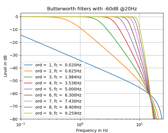
No, it's ambiguous. A Butterworth filter of any order can meet this requirement by choosing a cutoff frequency (which is the -3dB) point according to the order. See examples below

What is meant by "-60db at 20Hz"?

It means that a sine wave of 20 Hz would be attenuated by 60dB. Generally a lowpass filter passes low frequencies (hence the name) and attenuates higher frequencies.

Is it correct to use output='sos' and, subsequently, scipy.signal.sosfilt for smoothing this kind of data (6-dimensional IMU)?
Yes, that's best practice.

A Butterworth filter attenuates roughly 6dB/octave (= 20dB/decade) per order above the cutoff frequency. The higher the order, the steeper the slope. E.g. a 3rd order Butterworth filter has a slope of 18 dB/octave. We can use this to eyeball the required cutoff frequency to hit a -60dB frequency of $f_{60} = 20Hz$ as

$$f_c(o) = f_{60} \cdot 2 ^{-\frac{60}{6 \cdot o}}$$

where $o$ is the filter order

Here are the transfer functions of Butterworth lowpass filters of order 1 to 10 that have an attenuation of -60dB at 25 Hz ($f_s = 50Hz$)

enter image description here

$\endgroup$
3
  • $\begingroup$ Hmm... you should be able to get -60dB @ 25Hz (actually about 24.995Hz) with a first order LPF as well: `w0 = 2*pi*(20/50); a0 = cos(w0) + sin(w0) + 1.0; a1 = sin(w0) - cos(w0) - 1.0; b0 = sin(w0); b1 = sin(w0); a = [a0 a1]; b = [b0 b1]; FLT=tf(b, a, 1/fs); $\endgroup$
    – Juha P
    Commented Jun 5 at 20:32
  • $\begingroup$ @JuhaP: that gives -3dB at 20 Hz, not -60dB. $\endgroup$
    – Hilmar
    Commented Jun 6 at 17:09
  • $\begingroup$ yep, it does but, I commented sentence "Here are the transfer functions ... -60dB at 25Hz (fs=50Hz)" in your answer. Doesn't your plot show ~ -60dB @ 15Hz (if I read the plot properly). $\endgroup$
    – Juha P
    Commented Jun 8 at 8:46

Your Answer

By clicking “Post Your Answer”, you agree to our terms of service and acknowledge you have read our privacy policy.

Not the answer you're looking for? Browse other questions tagged or ask your own question.