1
$\begingroup$

I want a digital IIR filter with f0=225kHz and fs=53.125GHz. I can come up with the transfer function and plot it using Matlab. The problem arises when I try to do my own code that implements the filter instead of Matlab's filter() function.

Step 1

%Define transfer function
lpf_f0 = 225e3;
fs = 53.125e9;
tau = 1/(2*pi*lpf_f0 );
lpf_num = 1;
lpf_den = [tau 1];

%CT-DT conversion
[lpf_numd,lpf_dend] = bilinear(lpf_num, lpf_den, fs);

%Bode Plot
h_lpf= tf(lpf_numd,lpf_dend, 1/fs);
bopts = bodeoptions;
bopts.FreqUnits = 'Hz';
bopts.PhaseVisible = 'off';
bode(h_lpf, bopts)

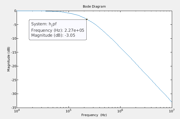
enter image description here

So far so good. Next, take a look at the time-domain response

Step 2

data = zeros(2^30,1);
data(100) = 1;
lpf_out_filt = filter(lpf_numd,lpf_dend, data);

figure(); 
plot((0:200000-1)/fs, lpf_out_filt(1:200000))
xlabel('Time [s]')
ylabel('Response')
title('LPF Time Domain Response')

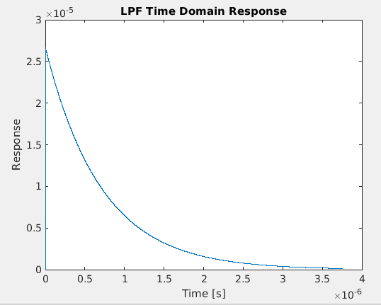
enter image description here

As expected, there's a really long tail. Good. Now let's do an FFT to cross-check the frequency response.

Step 3

lpf_out_cplx = fftshift(fft(lpf_out_filt));
f_step = fs/length(lpf_out_cplx);

lpf_out_cplx  = lpf_out_cplx(length(lpf_out_cplx)/2:end);
lpf_out_mag = abs(lpf_out_cplx);
lpf_out_freq = (1:length(lpf_out_mag))*f_step;

lpf_out_mag = 20*log10(lpf_out_mag);

i_f0 = find(lpf_out_mag<=-3,1);

figure();
semilogx(lpf_out_freq(1:i_f0*10), lpf_out_mag(1:i_f0*10))
title('LPF Response')
xlabel('Frequency [Hz]')
ylabel('Magnitide (dB)')
text(lpf_out_freq(i_f0), lpf_out_mag(i_f0), 'x')

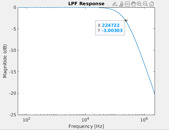
enter image description here

Still looking good. -3dB point is at 224.57kHz. This tells me that the above time-domain response is what I want to get the desired frequency-domain response.

Step 4

Now, the trouble comes when I try to do my own implementation instead of using filter(). I take the transfer function and come up with the difference equation:

>> h_lpf

h_lpf =
 
  1.331e-05 z + 1.331e-05
  -----------------------
           z - 1
 
Sample time: 1.8824e-11 seconds
Discrete-time transfer function.

Seems straighforward, but this is where things start to to awry

Multiply by numerator and denominator by z^-1 to get it in a causal form:

  1.331e-05 z + 1.331e-05       1.331e-05  + 1.331e-05 z^-1
  -----------------------  ==   -----------------------
           z - 1                        1 - z^-1

Difference equation is thus: y[n] = 1.331e-05*x[n] + 1.331e-05*x[n-1] + y[n-1]

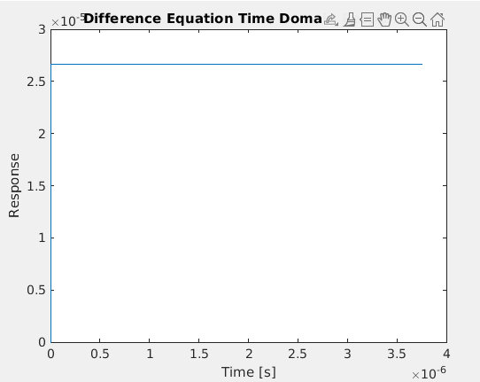
Intuitively, I can see that above equation is really just an integrator. An integrator won't yield the desired LPF response. There needs to be some coefficient applied to the y[n-1] other than 1 to yield the decay in the impulse response. Sure enough, I get a step-like response to a input pulse:

lpf_out = zeros(size(data));
lpf_out(1) = data(1)*lpf_numd(1);
for i=2:length(data)
    lpf_out(i) = lpf_numd*data(i-1:i) + lpf_out(i-1);
end

figure(); 
plot((0:200000-1)/fs, lpf_out(1:200000))
xlabel('Time [s]')
ylabel('Response')
title('Difference Equation Time Domain Response')

enter image description here

I know I need a different coefficient on the y[n-1]. Something related to the numerator coefficients seems pomising. Thinking about how a LPF (with 0dB gain at DC) will respond to a DC signal, I know the stead-state output will be the same as the input:x[n]=y[n] Assuming the input is a long string of 1's. Every filter iteration is adding 2*1.331e-05 on account of the 1.331e-05*x[n] + 1.331e-05*x[n-1] in the difference equation. The output will increase unbounded unless the y[n-1] is scaled.

Consider the case where the input is just 1's and the output is already at the known correct stead-state: y[n-1] = 1. To make sure the output stays at y[n]=1 in the presence of the 1.331e-05*x[n] + 1.331e-05*x[n-1] feed-forward contriubtion, the recursive contribution must be 1-2*1.331e-05. Thus we end up here:

y[n] = 1.331e-05*x[n] + 1.331e-05*x[n-1] + (1-2*1.331e-05)*y[n-1]

lpf_out = zeros(size(data));
lpf_out(1) = data(1)*lpf_numd(1);
for i=2:length(data)
    lpf_out(i) = lpf_numd*data(i-1:i) + lpf_out(i-1)*(1-sum(lpf_numd));
end

figure();
plot((0:200000-1)/fs, lpf_out(1:200000))
xlabel('Time [s]')
ylabel('Response')
title('Difference Equation Time Domain Response')

Sure enough, this yeilds the same time-domain response that the filter() approach in Step 3. However, why didn't I get here when I initially tried to derive the difference equation from the transfer function? Was I misinterpreting the transfer function or misunderstanding how to derive the difference equation?

$\endgroup$
3
  • $\begingroup$ Am I reading this right? 53 GHz? $\endgroup$ Commented Sep 4, 2021 at 10:00
  • $\begingroup$ None of the answers so far go into why you might want to be careful of rounding error, and under what circumstances -- without cluttering your question up with answers to things you didn't ask, I strongly suggest you find some reading material, or study up on your own, the sensitivity of polynomial roots to their coefficients, and why this has an impact on IIR filter design. Bottom line -- as the filter order goes up, and as the roots get closer to the unit circle, the required precision of the coefficients and data paths goes up, often drastically. $\endgroup$
    – TimWescott
    Commented Sep 4, 2021 at 16:18
  • $\begingroup$ Yes, it's a crazy low cut-off. I haven't fully baked what the final hardware implementation would look like. For my application, the accuracy of this filter isn't really that important. This question came from the "will this even work in theory" phase of the design. $\endgroup$
    – capj
    Commented Sep 5, 2021 at 23:24

2 Answers 2

1
$\begingroup$

this is where things start to to awry

Actually, no. Here's where things go sideways:


h_lpf =
 
  1.331e-05 z + 1.331e-05
  -----------------------
           z - 1
 
Sample time: 1.8824e-11 seconds
Discrete-time transfer function.

Or, rather, where you see what Matlab has printed out, and you take it for truth.

It's pretty obvious that the z - 1 in your denominator is really "z minus something that's been rounded to one".

I don't know the details of extracting a transfer function from Matlab (I don't use it for signal processing). But you need to figure out how to print out the numerator and denominator of that transfer function as arrays, and then you need to make sure you're printing them at full resolution. I think you'll find (as you figured out on your own) that it's really z - (1 - 2 * 1.331e-5).

$\endgroup$
2
  • $\begingroup$ Thanks, this may be the winner. I'll confirm tonight or tomorrow. I'd though Matlab typically would, by default, display a value rounded to 1 as "1.000" or something along those lines. I guess that does not apply for pretty printed transfer functions.` $\endgroup$
    – capj
    Commented Sep 5, 2021 at 23:14
  • $\begingroup$ Yep... K>> format long K>> lpf_dend lpf_dend = 1.000000000000000 -0.999973389216300 $\endgroup$
    – capj
    Commented Sep 5, 2021 at 23:30
1
$\begingroup$

Tim has it correct, it's a rounding error.

You have a very low cutoff frequency, which means that your pole will extremely close to the unit circle (or $ z= 1$) in this case and you need to practice good numerical "hygiene" so to speak. Working with rounded numbers is not going to work here, you need "exact" within the limit of your number format.

In your case lpf_dend(2) is $-0.999973389216300$. Apparently the display of tf() rounds that to $-1$ which puts the pole directly on the unit circle and makes the filter unstable.

That fix is easy to do though. You have already calculated the filter coefficients as [lpf_numd,lpf_dend] = bilinear(...). So the filter code (in the loop) becomes simply

  y(i) = lpf_numd(1)*x(i)+lpf_numd(2)*x(i=1)-lpf_dend(2)*y(n-1);

Technically you would to divide by 'lpf_dend(1)' but bilinear always normalizes the filter coefficients to $a_0=1$

$\endgroup$
2
  • $\begingroup$ I'll confirm for myself later, but that looks correct. Not referencing lfp_dend in my code was sloppy and caused a lot of wheel-spinning. Many thanks for your help! $\endgroup$
    – capj
    Commented Sep 5, 2021 at 23:17
  • $\begingroup$ Yep, this is it. I considered putting the lpf_dend(2) in the loop code a few times and just didn't do it. Instead, I spent an embarassing amount of time trying to debug in other directions. $\endgroup$
    – capj
    Commented Sep 5, 2021 at 23:35

Your Answer

By clicking “Post Your Answer”, you agree to our terms of service and acknowledge you have read our privacy policy.

Not the answer you're looking for? Browse other questions tagged or ask your own question.