Goal:
I have an unknow dynmical system $G(s)$ and I want to find it from measurement data, output $y(t)$ and input $u(t)$. The data is frequency responses.
Method:
I begun first with creating the data.
$$u(t) = A sin(2\pi \omega (t) t) $$
Where $\omega(t)$ is frequency in Hz over time and $A$ is fixed amplitude. Let's say that we know our model, just to make our data inside the computer.
t = linspace(0.0, 50, 2800);
w = linspace(0, 100, 2800);
u = 10*sin(2*pi*w.*t);
G = tf([3], [1 5 30]);
y = lsim(G, u, t);
Now when we have our data $u(t)$ and $y(t)$ and also $\omega(t)$. We can use Fast Fourier Transform to estimate the model.
First we find the complex ratio between $u(t)$ and $y(t)$ in frequency domain.
$$G(z) = \frac{FFT(y(t))}{FFT(u(t))}$$
  % Get the size of u or y or w
  r = size(u, 1);
  m = size(y, 1);
  n = size(w, 2);
  l = n/2;

  % Do Fast Fourier Transform for every input signal
  G = zeros(m, l*m); % Multivariable transfer function of magnitudes
  for i = 1:m
    % Do FFT
    fy = fft(y(i, 1:n));
    fu = fft(u(i, 1:n));

    % Create the complex ratios between u and y and cut it to half
    G(i, i:m:l*m) = (fy./fu)(1:l); % This makes so G(m,m) looks like an long idenity matrix
  end

  % Cut the frequency into half too and multiply it with 4
  w_half = w(1:l)*4;
Wee need to divide it into half due to frequencies have mirrors.
Now when we got our complex ratios. We need to create a discrete transfer function on this form:
$$G(z^{-1}) = \frac{B(z^{-1})}{A(z^{-1})}$$
$$A(z^{-1}) = 1 + A_1 z^{-1} + A_2 z^{-2} + A_3 z^{-3} + \dots + A_p z^{-p}$$ $$B(z^{-1}) = B_0 + B_1 z^{-1} + B_2 z^{-2} + B_3 z^{-3} + \dots + B_p z^{-p}$$
Where $p$ is the model order.
Now we are going to solve this as least squares.
$$A(z^{-1})G(z^{-1}) = B(z^{-1})$$
$$G(z^{-1}) = -A_1G(z^{-1})z^{-1} - \dots -A_pG(z^{-1})z^{-p} + B_0 + B_1 z^{-1} + \dots + B_p z^{-p}$$
Like this: $$ \begin{bmatrix} G(z_1^{-1})z_1^{-1} & \dots & G(z_1^{-1})z_1^{-p} & 1 & z_1^{-1} & \dots & z_1^{-p} \\ G(z_2^{-1})z_2^{-1} & \dots & G(z_2^{-1})z_2^{-p} & 1 & z_2^{-1} & \dots & z_2^{-p} \\ G(z_3^{-1})z_3^{-1} & \dots & G(z_3^{-1})z_3^{-p} & 1 & z_3^{-1} & \dots & z_3^{-p} \\ \vdots & \vdots & \vdots & \vdots & \vdots \\ G(z_l^{-1})z_l^{-1} & \dots & G(z_l^{-1})z_l^{-p} & 1 & z_l^{-1} & \dots & z_l^{-p} \end{bmatrix}$$
$$ \begin{bmatrix} -A_1\\ \vdots \\ -A_p\\ B_0\\ B_1\\ \vdots \\ B_p \end{bmatrix}$$
$$ = \begin{bmatrix} G(z_1^{-1})\\ G(z_2^{-1})\\ G(z_3^{-1})\\ \vdots \\ G(z_l^{-1}) \end{bmatrix}$$
Where $z_i = e^{j\omega_i T}$ where $T$ is the sample ratio of measurement.
Let's call this equation above for $Ax=B$
MATLAB / Octave code for that:
  Gz = repmat(G', 1, p);
  Ir = repmat(eye(r), l, 1); % Just a I column for size r and length l
  Irz = repmat(eye(r), l, p);
  for n = 1:l
    for j = 1:p
      z = (exp(1i*w_half(n)*sampleTime)).^(-j); % Do z = (e^(j*w*T))^(-p)
      sn = (n-1)*m + 1; % Start index for row
      tn = (n-1)*m + m; % Stop index for row
      sj = (j-1)*m + 1; % Start index for columns
      tj = (j-1)*m + m; % Stop index for columns
      Gz(sn:tn, sj:tj) = Gz(sn:tn, sj:tj)*z;    % G'(z^(-1))*z^(-1)
      Irz(sn:tn, sj:tj) = Irz(sn:tn, sj:tj)*z;  % Ir*z^(-1)
    end
  end
  % Join them all
  A = [Gz Ir Irz];
Now I going to solve this equation. We need to take accound that there are only complex values here. So we will solve this as:
$$\begin{bmatrix} real(A)\\ imag(A) \end{bmatrix}x = \begin{bmatrix} real(B)\\ imag(B) \end{bmatrix}$$
  Ar = real(A);
  Ai = imag(A);
  Gr = real(G');
  Gi = imag(G');
  A = [Ar; Ai];
  B = [Gr; Gi];
  x = (inv(A'*A)*A'*B)'; % Ordinary least squares
And the numerator and denominator from $x$ is
  den = [1 (x(1, 1:p))] % -A_1, -A_2, -A_3, ... , -A_p
  num = (x(1, (p+1):end)) % B_0, B_1, B_2, ... , B_p
And here is the problem.
The variable $den$ have poles that are larger than 1 in unit circle. That' means that the model is unstable.
Question:
What have I missed? What need to be done?
I assume that the least squares was not made correct. Right?
What I have checked:
I have checked that this code is correct:
  % Get the size of u or y or w
  r = size(u, 1);
  m = size(y, 1);
  n = size(w, 2);
  l = n/2;

  % Do Fast Fourier Transform for every input signal
  G = zeros(m, l*m); % Multivariable transfer function of magnitudes
  for i = 1:m
    % Do FFT
    fy = fft(y(i, 1:n));
    fu = fft(u(i, 1:n));

    % Create the complex ratios between u and y and cut it to half
    G(i, i:m:l*m) = (fy./fu)(1:l); % This makes so G(m,m) looks like an long idenity matrix
  end
Because I can plot the bode diagram of the measurement data
  % Cut the frequency into half too and multiply it with 4
  w_half = w(1:l)*4;

  % Plot the bode diagram of measurement data - This is not necessary for identification
  if(w_half(1) <= 0)
    w_half(1) = w_half(2); % Prevent zeros on the first index. In case if you used w = linspace(0,...
  end
  semilogx(w_half, 20*log10(abs(G))); % This have the same magnitude and frequencies as a bode plot
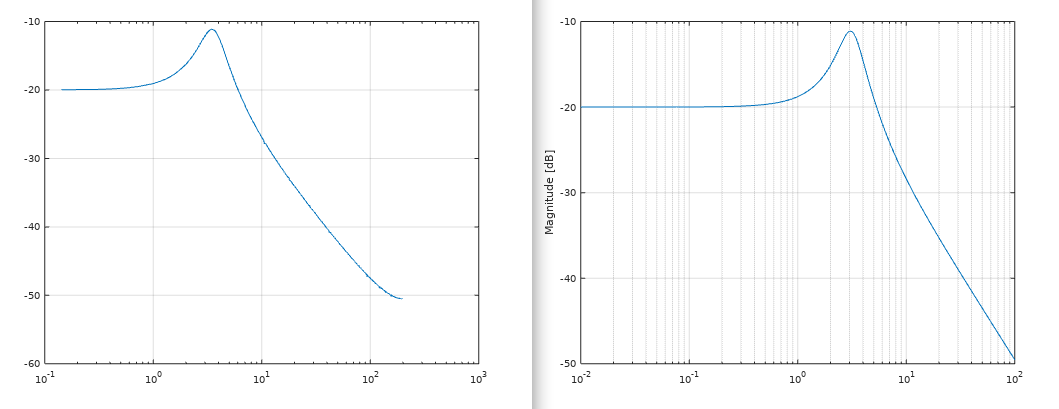
Assume that our model is
$$G(s) = \frac{3}{s^2 + 5s + 30}$$
There fore our bode diagram from data is going to look like this. The left picture shows the data-bode diagram and the right picture shows the bode diagram from the transfer function model.
You can follow the math logic at equation 14 here: https://ntrs.nasa.gov/archive/nasa/casi.ntrs.nasa.gov/19920023413.pdf


z = (e^(j*w*T))^(-p)or can I remove the negative sign?z = (e^(j*w*T))^p = e^(j*w*p*T)? What do you think? $\endgroup$