I have a discrete function that represents a 1d position in space over time. I have a motion system that would like to achieve this curve, but, due to constraints on jerk (3rd derivative) and acceleration (2nd derivative), it cannot actually achieve the motion. This occurs due to a discontinuity in the function, where it goes from a flat signal to a sharp rise.
I'm looking for an algorithm that will take the discrete series and produce a new series that approximates the original, without violating the upper limits on the magnitude of the second and third derivatives. I don't have a strict definition for how I'd like to minimize the error for the position, but a standard sum mean-squared error fit is probably reasonable. For the derivative, I'm approximating using the standard centered difference $\frac{f(x+1)-f(x-1)}{(2{\Delta}t)}$.
I've tried simply applying the limits and driving toward the target position as fast as possible, but this is unstable (it doesn't properly consider the de-jerk and decel time and therefore overshoots the target and oscillates.) I've considered applying a repeated low-pass filter until the constraints are met, but this seems like a bit of a hack and I'm not convinced it will give me a very good fit. Is there some way to create a filter that specifically limits the derivatives of the signal?
A few additional notes:
The new series must have the same length as the original series. This motion occurs at the same time as another operation and the two are strictly synchronized. It is acceptable, however, if it can't achieve the final position within the constraints; this just means that the parallel operation is too aggressive for the motion to follow. This should not occur, in practice, when configured properly.
I've started investigating an iterative approach that identifies a point that violates the constraints, then adjusts for the error and splits the negative of the error between the two neighboring points, so that the sum of the function values will be preserved. It then computes the error at the neighbor and transfers the remaining error to the left or right, respectively. If it reaches the end of the function and there is still error, it just chops to the limits. I don't know if this approach has any sound theoretical grounding, but I'll experiment and see how it performs with my signals.
More notes:
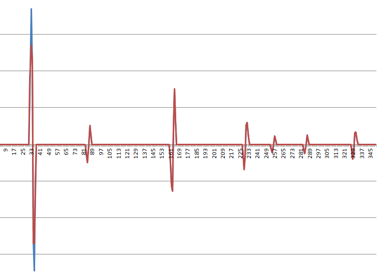
It's reasonable to approximate the jerk (third derivative) function as a linear combination of non-overlapping step and impulse functions. For a typical input series, it looks something like this (the blue vs. red is my current attempt at filtering; this is mainly just to convey an idea of the shape):

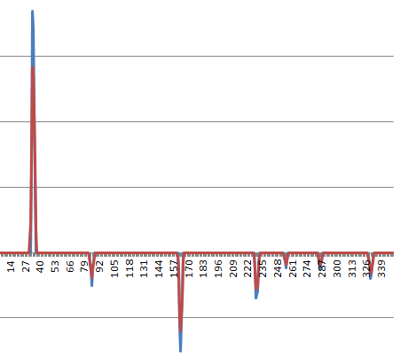
Here is a typical acceleration profile:

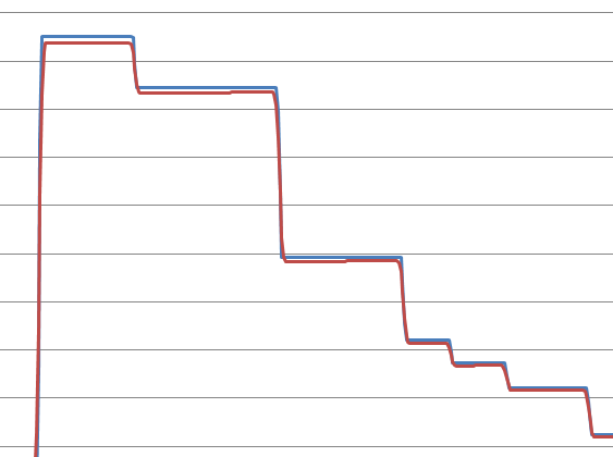
Here is a typical velocity profile (the climb at the start is what causes all the trouble; the physics of the problem make the system prefer to start moving at close to infinite velocity right from the get-go, but practical considerations get in the way):

For those who are interested, here is the raw tab-delimited data series from which the central-difference derivatives were approximated to produce the above graphs:
x 4.5 4.5 4.5 4.5 4.5 4.5 4.5 4.5 4.5 4.5 4.5 4.5 4.5 4.5 4.5 4.5 4.5 4.5 4.5 4.5 4.5 4.5 4.5 4.5 4.5 4.5 4.5 4.5 4.5 4.5 4.5 4.5 4.5 4.5 4.510544858 4.529570168 4.548595479 4.567620789 4.5866461 4.60567141 4.624696721 4.643722031 4.662747342 4.681772652 4.700797963 4.719823273 4.738848584 4.757873894 4.776899204 4.795924515 4.814949825 4.833975136 4.853000446 4.872025757 4.891051067 4.910076378 4.929101688 4.948126999 4.967152309 4.98617762 5.00520293 5.024228241 5.043253551 5.062278862 5.081304172 5.100329483 5.119354793 5.138380104 5.157405414 5.176430725 5.195456035 5.214481346 5.233506656 5.252531967 5.271557277 5.290582588 5.309607898 5.328633209 5.347658519 5.36668383 5.38570914 5.404734451 5.423759761 5.442785072 5.461810382 5.480714657 5.497626044 5.514537431 5.531448818 5.548360206 5.565271593 5.58218298 5.599094367 5.616005754 5.632917141 5.649828528 5.666739915 5.683651302 5.700562689 5.717474077 5.734385464 5.751296851 5.768208238 5.785119625 5.802031012 5.818942399 5.835853786 5.852765173 5.869676561 5.886587948 5.903499335 5.920410722 5.937322109 5.954233496 5.971144883 5.98805627 6.004967657 6.021879044 6.038790432 6.055701819 6.072613206 6.089524593 6.10643598 6.123347367 6.140258754 6.157170141 6.174081528 6.190992916 6.207904303 6.22481569 6.241727077 6.258638464 6.275549851 6.292461238 6.309372625 6.326284012 6.343195399 6.360106787 6.377018174 6.393929561 6.410840948 6.427752335 6.444663722 6.461575109 6.478486496 6.495397883 6.512309271 6.529220658 6.546132045 6.563043432 6.579954819 6.596866206 6.613777593 6.63068898 6.647600367 6.664511754 6.681423142 6.698334529 6.715245916 6.732157303 6.74906869 6.765980077 6.782891464 6.79783353 6.807698506 6.817563482 6.827428457 6.837293433 6.847158409 6.857023385 6.866888361 6.876753336 6.886618312 6.896483288 6.906348264 6.91621324 6.926078215 6.935943191 6.945808167 6.955673143 6.965538119 6.975403095 6.98526807 6.995133046 7.004998022 7.014862998 7.024727974 7.034592949 7.044457925 7.054322901 7.064187877 7.074052853 7.083917828 7.093782804 7.10364778 7.113512756 7.123377732 7.133242707 7.143107683 7.152972659 7.162837635 7.172702611 7.182567587 7.192432562 7.202297538 7.212162514 7.22202749 7.231892466 7.241757441 7.251622417 7.261487393 7.271352369 7.281217345 7.29108232 7.300947296 7.310812272 7.320677248 7.330542224 7.3404072 7.350272175 7.360137151 7.370002127 7.379867103 7.389732079 7.399597054 7.40946203 7.419327006 7.429191982 7.439056958 7.448921933 7.45668417 7.46311785 7.46955153 7.47598521 7.48241889 7.488852569 7.495286249 7.501719929 7.508153609 7.514587289 7.521020969 7.527454649 7.533888329 7.540322008 7.546755688 7.553189368 7.559623048 7.566056728 7.572490408 7.578924088 7.585357768 7.591791447 7.598225127 7.604658807 7.611092487 7.617471594 7.622952136 7.628432678 7.63391322 7.639393762 7.644874304 7.650354846 7.655835389 7.661315931 7.666796473 7.672277015 7.677757557 7.683238099 7.688718641 7.694199183 7.699679725 7.705160268 7.71064081 7.716121352 7.721601894 7.727082436 7.732562978 7.73804352 7.743524062 7.749004605 7.754485147 7.759965689 7.765446231 7.770926773 7.776407315 7.781828236 7.786267475 7.790706714 7.795145953 7.799585192 7.804024432 7.808463671 7.81290291 7.817342149 7.821781388 7.826220627 7.830659866 7.835099105 7.839538344 7.843977584 7.848416823 7.852856062 7.857295301 7.86173454 7.866173779 7.870613018 7.875052257 7.879491497 7.883930736 7.888369975 7.892809214 7.897248453 7.901687692 7.906126931 7.91056617 7.915005409 7.919444649 7.923883888 7.928323127 7.932762366 7.937201605 7.941640844 7.946080083 7.950519322 7.954958561 7.959397801 7.96383704 7.968276279 7.972715518 7.977154757 7.980384921 7.982851165 7.985317409 7.987783653 7.990249897 7.992716141 7.995182385 7.997648629 8.000114873 8.002581117 8.005047361 8.007513605 8.009979849 8.012446092 8.014912336 8.01737858 8.019844824 8.022311068 8.024777312 8.027243556 8.0297098 8.032176044 8.034642288 8.037108532 8.039574776 8.04204102 8.044507264 8.046973508 8.049439752 8.051905996 8.05437224 8.056838484 8.059304728 8.061633119 8.063606114 8.065579109 8.067552105 8.0695251 8.071498095 8.07347109 8.075444085 8.07741708 8.079390076 8.081363071 8.083336066 8.085309061 8.087282056 8.089255051 8.091228046 8.093201042 8.09410447 8.094332124 8.094559777 8.09478743 8.095015084 8.095242737 8.09547039 8.095698043 8.095925697 8.09615335 8.096381003 8.096608657 8.09683631 8.097063963 8.097291616 8.09751927 8.097746923 8.097974576 8.09820223 8.098429883 8.098657536 8.098885189 8.099112843 8.099340496 8.099568149 8.099795803 8.100023456 8.100251109 8.100478762 8.100706416 8.100934069 8.101161722 8.101389376 8.101617029 8.101844682 8.102072336 8.102299989 8.102527642 8.102755295 8.102982949 8.103210602 8.103438255 8.103665909 8.103893562 8.104121215 8.104348868 8.104576522 8.104804175 8.105031828 8.105259482 8.105487135 8.105714788 8.105942441 8.106170095 8.106397748 8.106625401 8.106853055 8.107080708 8.107308361 8.107536014 8.107763668 8.107991321 8.108218974 8.108446628 8.108674183 8.108899792 8.109120089 8.109331659 8.109531087 8.109714959 8.10987986 8.110022376 8.110139158 8.11022965 8.110297009 8.110344649 8.110375986 8.110394434 8.110403409 8.110406324 8.110406324
