Derive velocity and acceleration from position

Question

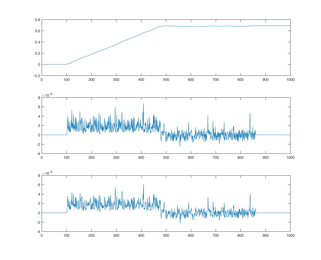
I generate random spike data that represent the ouput from a rotary encoder. Here the output of my algorithm: The first plot is position, then velocity and then acceleration. Even though I downsample my position vector and pass it to a average filter of 20 points, the derivative are very sensitive as you can see. I check the following question: have position, want to calculate velocity and acceleration. Few option seem to be available , but I don't get the answer , the Savitzky-Golay Filters is just a smoothing function, I don't get how he get the velocity, also what are the orther alternatives.

Answer 1

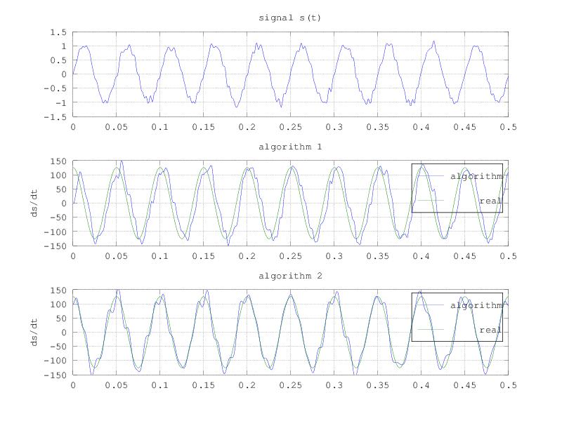
There are several ways to calculate the derivative of a stochastic signal. I will show you two methods.

First of all, adjust the output of a second order transfer function to your data: $${\omega_n^2}/({s^2+2\zeta\omega_n s+\omega_n^2})$$ Once you are satisfied with the fit, put an additional $s$ in the numerator and you will get the derivative of your signal: $${\omega_n^2\times s}/({s^2+2\zeta\omega_n s+\omega_n^2})$$ You can use a bilinear transformation and convert this solution into a discrete one, to implement in a software easily, if you like.

Another solution is to use the spectrum and calculate the fft of your signal. Then filter it vanishing the small values in the higher frequencies. Now, take the result and multiply it by $j\omega$. This is taken from the Fourier Transform Properties Table to calculate the derivative of a signal. Finally, redo the signal with ifft.

I added here a code to exemplify these aforementioned algorithms. The output picture is added as well at the end of the post. I hope it helps.

% \brief: this code exemplifies two techniques suitable for
%         calculating the first-order derivative of an
%         stochastic signal.
%
% \algorithm 1: LTI transfer function integrated with Tustin.
% \algorithm 2: FFT derivative property.
%
% \author:     Luciano Augusto Kruk
% \web:        www.kruk.eng.br

% some constants:
fs = 1000; % [Hz] sample rate
T  = 1/fs;
t  = 0:T:0.5;
nT = length(t);
% signal + colored noise:
[B,A] = butter(10,250*T*2);
s     = sin(2*pi*20*t)+filter(B,A,0.1*randn(1,nT));

figure(1); clf;
subplot(3,1,1);
plot(t,s);
title('signal s(t)');
grid on;

% first technique: second order transfer function
qsi  = 0.7;
wn   = 2*pi*60;
wnT2 = (wn*T)^2;
b    = 2*T*wn*wn;
a1   = 4 + (4*qsi*wn*T) + wnT2;
a2   = (2*wnT2)-8;
a3   = wnT2 - (4*qsi*wn*T) + 4;
dsdt = zeros(size(s));
for i = 3:nT
    dsdt(i) = (1/a1) * ...
        ((-a2*dsdt(i-1)) - (a3*dsdt(i-2)) + (b * (s(i) - s(i-2))));
end
subplot(3,1,2);
plot(t,dsdt, t,2*pi*20*cos(2*pi*20*t))
title('algorithm 1');
ylabel('ds/dt');
grid on;
set(gca, 'ylim', 150*[-1 1])
legend('algorithm', 'real')

% second technique: fft/ifft properties
s_fft = fft(s);
idx   = 1:(nT/2);
f_fft = (idx-1) * (fs/2) * (1/length(idx));
idx   = round((nT/2) + ((-nT/2.5):(nT/2.5)));
s_fft(idx) = 0;
w     = 2*pi*(((-nT/2):((nT/2)-1))/nT)*fs;
dsdt  = ifft(s_fft .* sqrt(-1) .* ifftshift(w));

subplot(3,1,3);
plot(t,dsdt, t,2*pi*20*cos(2*pi*20*t))
title('algorithm 2');
ylabel('ds/dt');
grid on;
set(gca, 'ylim', 150*[-1 1])
legend('algorithm', 'real')