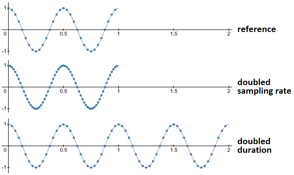
In summary,
- Doubled duration: $f$ doubled
- Doubled sampling rate: $f$ unchanged
- Non-zero $t[0]$: $\phi \rightarrow \phi + 2\pi f t[0]$ (using old $f$)
- Duration, sampling rate: $T = (t[1] - t[0])\cdot N$, $S = 1 / (t[1] - t[0])$, $S = N/T$
In one equation: $\texttt{sine_dft}\{N, fT, \phi + 2\pi f t[0]\}$. In SR terms, $fT \rightarrow f(N/S)$.
Effects on power/energy are described in Relationship between energy, power, and sampling rate?
Understanding SR vs Duration
Recall, the result's for
$$
\texttt{DFT}\{\cos(2\pi f t + \phi)\},
$$
where $t = \frac{1}{N}[0, 1, ..., N - 1]$. Let $N = 4$, so $t = [0, 0.25, 0.5, 0.75]$. We have:
- Doubled sampling rate: $\rightarrow [0, 0.125, 0.25, 0.375, 0.5, 0.625, 0.75, 0.875]$. So, $N \rightarrow 2N$ and $f$ unchanged, hence $(f / N) \rightarrow (f / N) / 2$. Note, despite the $0.875$, the duration hasn't changed; for $N \rightarrow \infty$, the last sample approaches $1$. This can be proven (without the $\infty$).
- Doubled duration: $\rightarrow [0, 0.25, 0.5, 0.75, 1, 1.25, 1.5, 1.75]$. So, $N \rightarrow 2N$, and now since there's twice the total oscillations, $f \rightarrow 2f$. Hence, $f/N$ is unchanged.
For spectral analysis, it can be more useful to reformulate these in terms of least possible change in DFT and signal, while staying equivalent in discrete terms. That would be:
- Doubled sampling rate: $f \rightarrow f/2$, unchanged $N$. Same DFT, but now the sine is halved in frequency.
- Doubled duration: $N \rightarrow 2N$, unchanged $f/N$. Same sine, but now the DFT has twice the samples.
For analyzing the effects on a reference signal, it's more useful to think of what actually happens with the parameters; that's in the first version. Expressed parametrically (follows first version),
$$
\begin{alignat}{1}
\text{Sampling rate:}\ \
& f_\text{new} &= f_\text{old}\quad
& N_\text{new} = N_\text{old} (S_\text{new} / S_\text{old}) \\
\text{Duration:}\ \
& f_\text{new} &= f_\text{old} (T_\text{new} / T_\text{old}) \quad
& N_\text{new} = N_\text{old} (T_\text{new} / T_\text{old})
\end{alignat}
$$
Visually (follows first version),

Note, the DFT will not "see" the doubled duration plot, i.e. $t \in [0, 2]$; its domain always spans a unit interval, and everything else re-expresses itself around it to attain equivalence, hence the "spectral analysis" perspective. Below section extends this one.
Effects on parameters
We could express a sine DFT solution purely in terms of sampling rate and duration, but it suffices, and is useful and much simpler, to simply understand how $f, N, \phi$ change with changes in physical characteristics. Of course, here, $t$ must be uniform (all $t[n] - t[n - 1]$ same).
Let $S = \text{sampling rate}$, $T = \text{duration}$, hence $t = [t_0, t_0 + 1/S, ..., t_0 + 1/S\cdot(N - 1)]$ or (same) $t = [t_0, t_0 + T/N, ..., t_0 + T/N\cdot(N - 1)]$. Some info repeats the previous section.
- $f \rightarrow f\cdot T$: doubled duration means doubled the wiggles - DFT's $f$ counts the wiggles
- $f \rightarrow f (N/S)$ per previous, since $T = N/S$
- $\phi \rightarrow \phi + 2\pi ft_0$: starting at $t_0$ is same as time-shifting to $t_0$: $\cos(2\pi f t + \phi)=$ $\cos(2\pi f (t' + t_0) + \phi)$, where $t' = [0, 1/S, ..., (N-1)/S]$. Expanding second's arg-ument, $2\pi f t' + 2\pi ft_0 + \phi$; this matches the original solution's formulation, with the sub.
- $T \neq t[-1] - t[0]$, and $S \neq N/(t[-1] - t[0])$. Common pitfalls. The duration is tricky - see below, also explained here.
Code validation & illustration
Illustrates above points, and shows equivalence of different constructions of $t$. sine_dft is found here.
import numpy as np
from numpy.fft import fft

# configure
N, f, phi, t0, S = (128, 3.5, 1.1, 3.5, 12.9)

# make time vector; show from all major perspectives
t = np.zeros(N)
t[0] = t0
for n in range(1, N):
    t[n] = t[n - 1] + 1/S
assert np.allclose(t, np.linspace(t0, t0 + N/S, N, endpoint=False))
assert np.allclose(t, np.arange(start=t0, stop=t0 + N/S, step=1/S))

# make sine
x = np.cos(2*np.pi * f * t + phi)

# show how we retrieve parameters
S = 1 / (t[1] - t[0])
T = N / S
f_adj = f * T
phi0 = phi + 2*np.pi*f*t[0]

# assert equality
xf0 = sine_dft(N, f_adj, phi0)
xf1 = fft(x)
assert np.allclose(xf0, xf1)
Effect on general signal
- Increased sampling rate: "refines" the existing spectrum by reducing leakage / aliasing, without necessarily changing peaks' location. If original SR was below Nyquist (exact or "effective"), then peak locations${}^1$ may change. For any amount of aliasing, the "effective" peak location (e.g. as mean of a few peaks) will almost always change, but negligibly if we're sufficiently above "effective Nyquist" - this happens very quickly for sines.
- Increased duration: this could mean one of two things:
- Underlying function is sampled over a greater interval: anything could happen, new contents are introduced (almost anything). If "new" exactly repeats "original", that's periodicity and inserts zeros between existing DFT bins. If "new" samples a function that repeats, e.g. sine, then peak locations are moved up by approximately $T_\text{new}/T_\text{orig}$ (only the newly-sampled interval must "repeat").
- Original signal is stretched out over a longer interval: the DFT doesn't care, this is identical to increased sampling rate.
1: for sines, SR still doesn't change $f$. In short, $fT$ remains valid for $\texttt{sine_dft}$, even if below Nyquist, and $k' = \pm f_d$ remains true, where $k'$ is continuous and maps to the underlying function that $k$ is sampling (the sine solution), and $f_d$ is $fT$ after accounting for $N/2$-modularity ("wrap"). SR changes $f_d$ if going from below to above Nyquist. $f_d$ is always recoverable exactly (see sine solution Q&A), and it matches $fT$ if above Nyquist, else it can be matched with more info.

