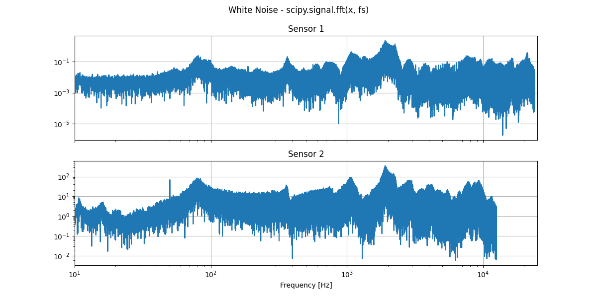
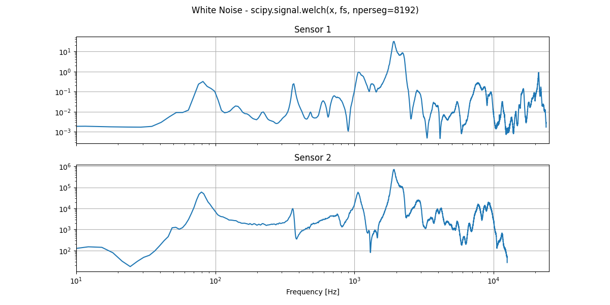
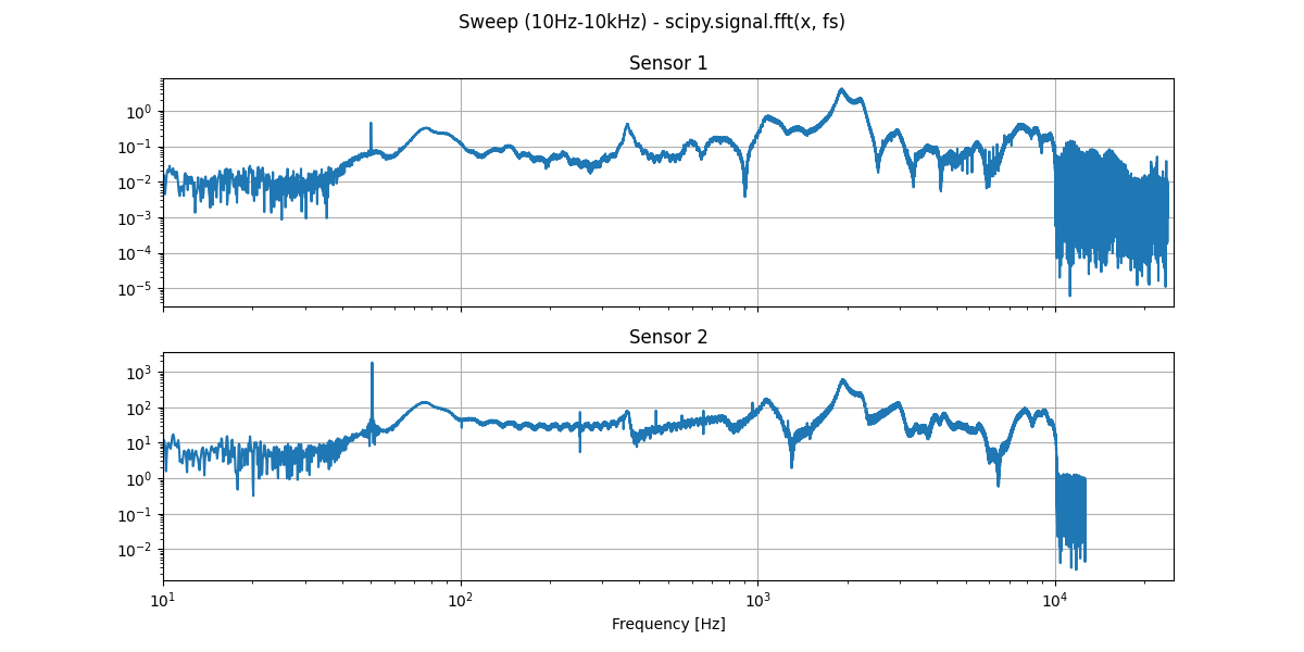
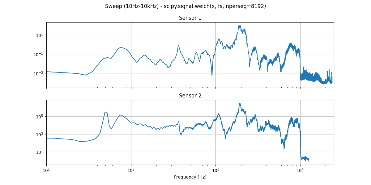
I will address the questions first and then I have a suggested additional approach that could be considered based on well established channel estimation techniques used in wireless communications (which this seems to parallel well). However given my attempts I only see a way to optimally determine the combined difference in the frequency response of both sensors but am not able to uniquely resolve each sensor without the use of a calibrated loudspeaker or calibrated sensor. With the use of such calibrated equipment, the techniques described here have value for practical channel estimation and frequency response determination.
Question 1: On the first glance the WhiteNoise- and Sweep-Plots look
pretty non-linear to me. But since Sensor 2 (the one with the known
linear response) is similar to Sensor 1 I suspect that most of the
nonlinearity comes from the signal source. Is this a reasonable
assumption?
First a clarification. Referring to the response as "non-linear" may cause confusion since the term non-linear with reference to systems means that the output will produce additional frequencies not present in the inputs. A non-linear system will produce integer harmonics given a single tone at the input. For the most part from the single tone measurements we see that we can consider the system to be linear. If we did see non-linear effects, it typically means that we are over-driving the input (which can also feasibly happen), and for doing such testing, we need to lower the input signal level. For signal-to-noise purposes, we do want to drive the signal as hard as we can while still being linear and thus achieve the best estimate of the result.
I believe you mean the response is "flat" or constant across frequency, or perhaps smooth with a "linear" slope versus frequency on a log plot (and hence "linear" vs "non-linear"). This is possible although how did you really establish that sensor 2 is flat or smooth, and would be with this measurement approach if the source was known to be linear? Could this be a misleading assumption?
Question 2: Can I use this data to actually calculate the frequency
response of sensor 1? (e.g. Sensor 2 is known -> calculate frequency
response of signal source -> calculate frequency response of Sensor 1)
IF the frequency response of sensor 2 was confidently known, then yes. The approach to use sensor 2 as a "standard" and ultimately calibrate the source which is then used to measure sensor 2. For this we would need to be confident in the results of sensor 2, and confident in the connection between the source and sensor 1 is sufficiently identical to the connection between the source and sensor 2. Further, we can remove the small frequency offset errors with the uncorrelated sample rates by comparing the sample 1 and sample 2 outputs for the same tone at the input. This comparison is best done with correlation techniques which is further expanded on in my additional suggestions.
Question 3: Are there any flaws/pitfalls with my approach? E.g.
literature suggests checking the coherence (magnitude squared
coherence) in similar cases.
Yes I agree that coherence techniques would be best, which is what I will further detail below using channel estimation techniques.
Suggested Approach for Characterizing the Sensor Frequency Response
Please first see these posts on using the Wiener Hopf equations for least squares channel estimation for linear channels (and here linear I mean by definition what I clarified above).
Compensating Loudspeaker frequency response in an audio signal
How determine the delay in my signal practically
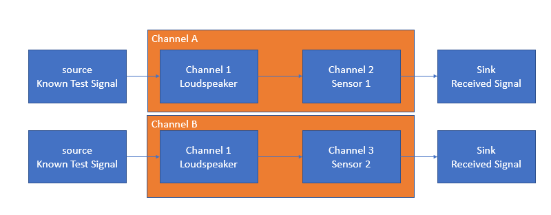
The above posts detail with usable code how to use the Wiener-Hopf equations for least squares channel estimation which essentially optimally (in a least-squares error sense) computes the inverse convolution to determine an unknown channel given a known test signal and known received signal. This is the same framework as the question here as suggested by the block diagrams below. In this case we have a known source ("test signal") and an unknown channel consisting of both the loudspeaker and each sensor in cascade which then results in the output waveform shown as the "received signal". I refer to the combined response of speaker and sensor as "Channel A" and "Channel B". With reference to the details in the referenced post, we are seeking in the time domain the impulse response of these channels (and the Fourier Transform of the impulse response is the frequency response). The known "test signal" will convolve with the unknown channel response and give us the known "received signal". Thus if we can solve for the inverse convolution, we can determine the unknown. The approach given does this with an overdetermined approach resulting in a classical least squares solution.

Some important points to stress in using this technique: It is very important that the source "Test Signals" be spectrally rich. White noise is perfect but it needs to be a known sample of white noise. Pseudo-random noise sequences are commonly used for this approach given we can easily repeat the test condition and provide a spectrally rich signal. If the source does not have energy in any given frequency, the solution can not be determined for that frequency. Testing with individual tones would then do this one frequency at a time, so would be a laborious and lengthy process versus a wide band test signal. The signal need not be perfectly flat (white) but the error of the result will be inversely proportional to the SNR at any given frequency so approaching a white noise source is optimum. Chirp signals (ramp frequency response) are also useful but can lead to further challenges with ensuring proper chirp rates compared to capture times.
Once "Channel A" and "Channel B" are determined (and I would repeat any process with modified test waveforms to assess repeatability and accuracy of the result), we consider that Channel A and Channel B (now known) have a common loudspeaker channel and different sensors which together form a convolution in the time domain, so we have the following relationships where $*$ represents a convolution operator:
$$h_A[n] = h_s[n]*h_1[n]$$
$$h_B[n] = h_s[n]*h_2[n]$$
Where:
$h_A[n]$: Impulse response of Channel A (known)
$h_B[n]$: Impulse response of Channel B (known)
$h_s[n]$: Impulse response of the loudspeaker (unknown)
$h_1[n]$: Impulse response of sensor 1 (unknown)
$h_2[n]$: Impulse response of sensor 2 (unknown)
We note from above that we have two equations with three unknowns ($h_s[n]$, $h_1[n]$, and $h_2[n]$) so from this we are only able to establish the difference of the two channels but not yet determine how much is allocated to each sensor. Noting that by using a third sensor (which the OP has mentioned in comment would be feasible), we may be able to resolve each sensor uniquely using approaches similar to "3 corner-hat characterization". This requires our ability to measures the difference between Sensor 1 and Sensor 2, Sensor 1 and Sensor 3 and Sensor 2 and Sensor 3. The approach detailed thus provides the difference measurement, and results in three equations and three unknowns suggesting that each channel can be uniquely determined.
I attempted to pursue this further as detailed below, but the resulting equation is singular with no solution. The 3 corner hat technique makes use of the statistical independence of the noise processes, which is not applicable here. I do not yet see a path of resolving the sensors uniquely without the additional use of either a calibrated loudspeaker or calibrated sensor, but will leave these thoughts in case the OP or anyone else is able to expand on a solution.
In the frequency domain, as the Fourier Transform of the measured channels given as $F_A(\omega)$, $F_B(\omega)$, and $F_B(\omega)$, we would have the following relationships (to make the equations less cumbersome, I omitted the $(\omega)$ but each are a function of $(\omega)$):
$$F_A = F_s F_1$$
$$F_B = F_s F_2$$
$$F_C = F_s F_3$$
From which we establish the "difference channels" mentioned above as (difference in dB units, but here we are using the direct product terms), with $F_{12}, F_{13}, F_{23}$ known:
$$F_{12} = \frac{F_A}{F_B} = \frac{F_1}{F_2}$$
$$F_{13} = \frac{F_A}{F_C} = \frac{F_1}{F_3}$$
$$F_{23} = \frac{F_B}{F_C} = \frac{F_2}{F_3}$$
 Power Spectral Density:
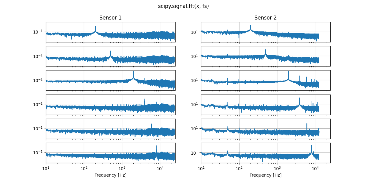
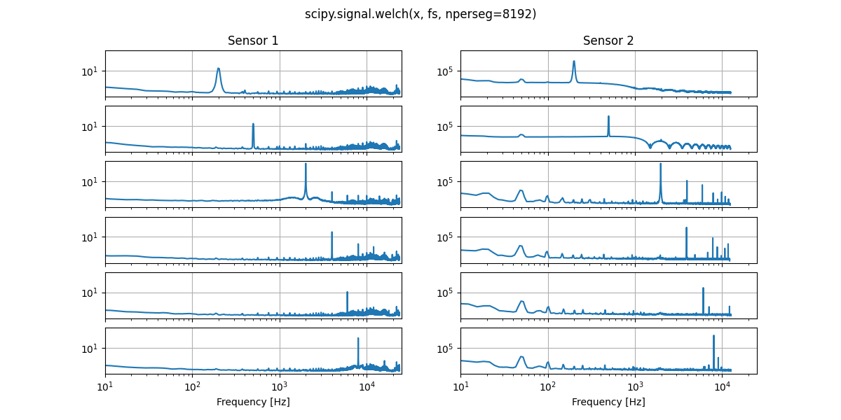 The subplot-rows correspond to the different frequencies of the frequency generator (200Hz, 500Hz, 2kHz, 4kHz, 6kHz, 8kHz).
Sensor 2 seems to pick up 50Hz noise but but for both sensors the generated frequency is clearly visible.
