I was looking into a technique called Random decrement technique from the following links/articles:
- How can I use Random Decrement Method to convert a non-stationary signal into a decay function using Matlab?
- Random Decrement Technique
- Using the Random Decrement Method for the Decentralized Acquisition of Modal Data
I found out that this technique was created in MATLAB which can be found in the following link (Damping ratio estimation from ambient vibrations (SDOF)). I tried to convert the code into python using smop, however, I think I made a mistake with the conversion. I feel that I misused smop package and tried recoding the converted file, but, I feel that I might have done something wrong. The code and conversion can be found below:
MATLAB:
function [R,t] = RDT(y,ys,T,dt)
%
% [R] = RDT(y,ys,T,dt) returns the free-decay response (R) by
% using the random decrement technique (RDT) to the time serie y, with a
% triggering value ys, and for a duration T
%
% INPUT:
%   y: time series of ambient vibrations: vector of size [1xN]
%   dt : Time step
%   ys: triggering values (ys < max(abs(y)) and here ys~=0)
%   T: Duration of subsegments (T<dt*(numel(y)-1))
% OUTPUT:
%   R: impusle response function
%   t: time vector asociated to R
%
% Author: E. Cheynet - UiB - last modified 14-05-2020
%%
if T>=dt*(numel(y)-1)
    error('Error: subsegment length is too large');
else
    % number of time step per block
    nT = round(T/dt); % sec
end
if ys==0
    error('Error: ys must be different from zero')
elseif or(ys >=max(y),ys <=min(y)),
    error('Error:  ys must verifiy : min(y) < ys < max(y)')
else
    % find triggering value
    ind=find(diff(y(1:end-nT)>ys)~=0)+1;

end
% construction of decay vibration
R = zeros(numel(ind),nT);
for ii=1:numel(ind)
    R(ii,:)=y(ind(ii):ind(ii)+nT-1);
end
% averaging to remove the random part
R = mean(R);
% normalize the R
R = R./R(1);
% time vector corresponding to the R
t = linspace(0,T,numel(R));
end

coeff = 5; % interpolation coefficient
newDT = median(diff(interp(t,coeff)));
newY = interp(y,coeff);
% triggering value
ys = max(abs(y))/5;
% subsegment duration
Ts = round(t(end)/30);

% RDT function
[IRF,newT] = RDT(newY,ys,Ts,newDT);
% get the envelop of the curve with the hilbert transform:
envelop = abs(hilbert(IRF));
envelop(1)=IRF(1);
clf;close all;
figure
hold on; box on;
plot(newT,IRF,'b',newT,envelop,'k');
xlabel('time (s)')
ylabel('normalized displacement')
xlim([0,Ts])
set(gcf,'color','w')
% fit an exponential decay to the envelop
optionPlot = 1;
wn = 2*pi*0.2; % -> obtained with peak picking method (fast way)
[zeta] = expoFit(envelop,newT,wn,optionPlot);
legend('IRF','envelop',' best fit')
Python:
# Generated with SMOP  0.41
# from libsmop import *
# RDT.m

from scipy.signal import chirp, spectrogram
import matplotlib.pyplot as plt
import numpy as np
from scipy.interpolate import interp1d


# @function
def RDT(y=None,ys=None,T=None,dt=None,*args,**kwargs):
    # varargin = RDT.varargin
    # nargin = RDT.nargin


    # [R] = RDT(y,ys,T,dt) returns the free-decay response (R) by
# using the random decrement technique (RDT) to the time series y, with a
# triggering value ys, and for a duration T

    # INPUT:
#   y: time series of ambient vibrations: vector of size [1xN]
#   dt : Time step
#   ys: triggering values (ys < max(abs(y)) and here ys~=0)
#   T: Duration of subsegments (T<dt*(np.size(y)-1))
# OUTPUT:
#   R: impusle response function
#   t: time vector asociated to R
#
# Author: E. Cheynet - UiB - last modified 14-05-2020

    if T >= np.dot(dt,(np.size(y) - 1)):
        error('Error: subsegment length is too large')
    else:
        # number of time step per block
        nT=round(T / dt)
# RDT.m:22

    if ys == 0:
        error('Error: ys must be different from zero')
    else:
        if ys >= max(y) or ys <= min(y):
            error('Error:  ys must verifiy : min(y) < ys < max(y)')
        else:
            # find triggering value
            ind=np.nonzero(np.diff(y(np.arange(1,y[-1] - nT)) > ys) != 0) + 1
# RDT.m:30

    # construction of decay vibration
    R=zeros(np.size(ind),nT)
# RDT.m:34
    for ii in np.arange(1,np.size(ind)).reshape(-1):
        R[ii,np.arange()]=y(np.arange(ind(ii),ind(ii) + nT - 1))
# RDT.m:36

    # averaging to remove the random part
    R=mean(R)
# RDT.m:39
    # normalize the R
    R=R / R(1)
# RDT.m:41
    # time vector corresponding to the R
    t=np.linspace(0,T,np.size(R))
# RDT.m:43
    return R,t

if __name__ == '__main__':
    t = np.linspace(0, 10, 3000)
    w = chirp(t, f0=6, f1=1, t1=10, method='linear')
    plt.plot(t, w)
    plt.title("Linear Chirp, f(0)=6, f(10)=1")
    plt.xlabel('t (sec)')
    plt.show()

    N = 3000 # number of time step
    # t = linspace(0,1800,N); # time
    dt = np.median(np.diff(t)) # time step
    fs = 1/dt

    coeff = 5 # interpolation coefficient
    newDT = np.median(np.diff(np.interp(coeff, t, w)))
    # newDT = np.median(np.diff(interp1d(t, t, w)))
    newY = np.interp(coeff, t, w)
    # triggering value
    ys = max(abs(w))/5
    # subsegment duration
    Ts = round(t[-1]/30)

    R, t = RDT(newY,ys,Ts,newDT)

    pass
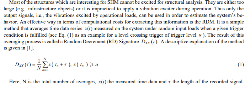
I want to obtain a function for RDT and fit the decreasing decrement using an envelope to make sure that it follows decreasing /impulse signal. What could be my mistake here and obtain a reasonable impulse signal? An equation for RD can be found in the following article and photo. (Design of a Random Decrement Method Based Structural Health Monitoring System)
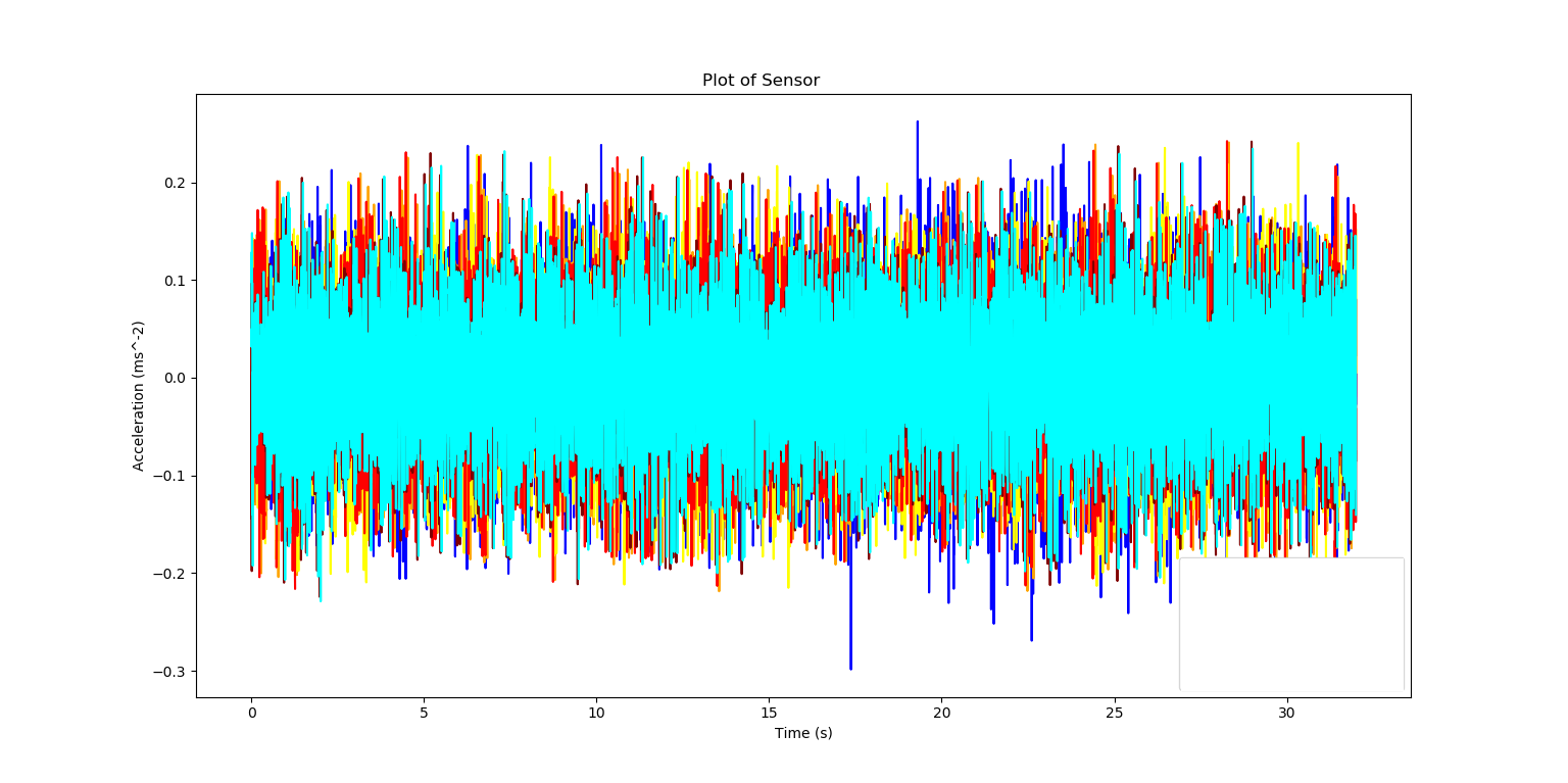
I want to implement the function onto for instance signals similar to the ones in the photo below.
The errors I am getting:
ind=np.nonzero(np.diff(y(np.arange(1,y[-1] - nT)) > ys) != 0) + 1
TypeError: 'numpy.ndarray' object is not callable


newDT = np.median(np.diff(np.interp(coeff, t, w)))
raise ValueError("diff requires input that is at least one dimensional")
ValueError: diff requires input that is at least one dimensional
Also, I’m mainly stuck at this line:
Python:
            # find triggering value
            ind=np.nonzero(np.diff(y(np.arange(1,y[-1] - nT)) > ys) != 0) + 1
MATLAB:
    % find triggering value
    ind=find(diff(y(1:end-nT)>ys)~=0)+1;
So, how would I convert this line for the find in MATLAB to python code?


