Object Detection using audible sonar

Question

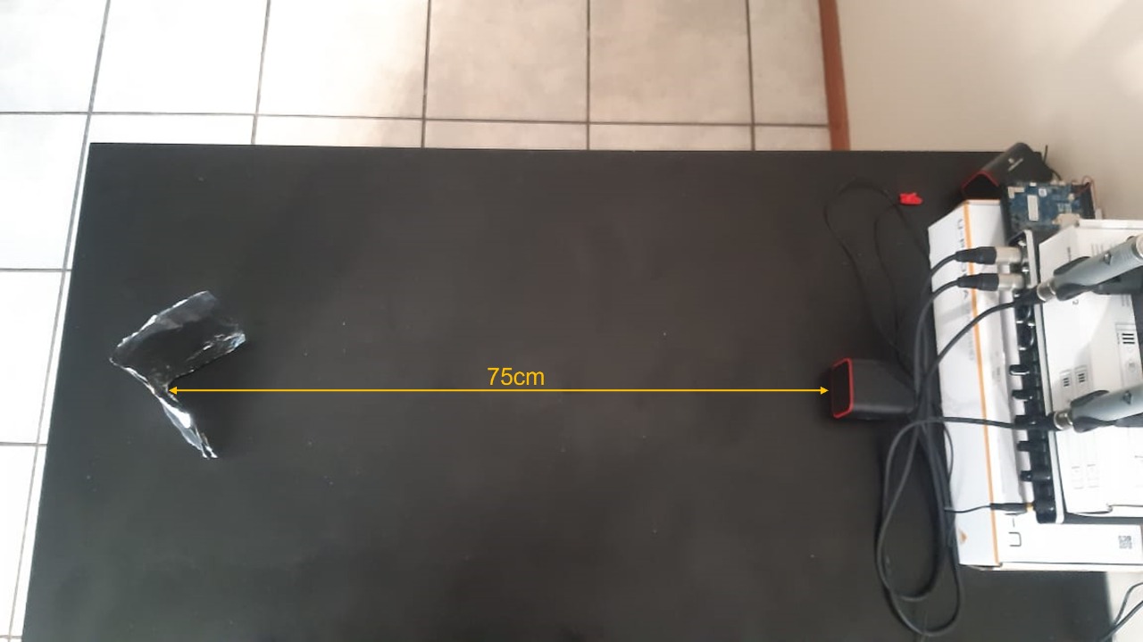
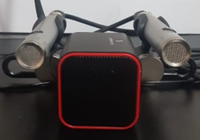
I am currently working on a project of identifying the position and angle of the objects in an environment using sonar (audible) about 1 to 2 m away from a desktop speaker within an angular sector of 60 degrees using some very powerful PreSonus PM-2 microphones and a Behringer UMD404HD.

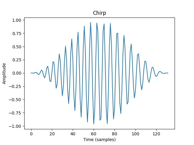
This is in PyCharm with Python3.6 interpreter. Using Audacity to record simultaneously as I play the chirp in the figure below:

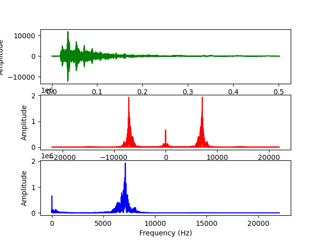
The following are results (Sound recording, FFT, single-sided FFT) I have obtained for a corner reflector placed ~75cm away from the sound source:

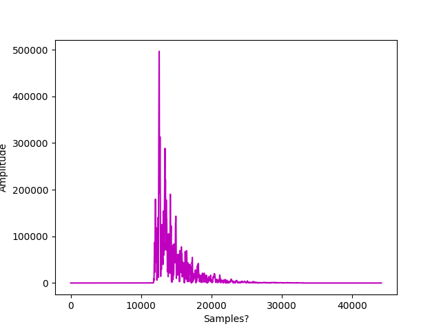
The next step is to apply a matched filter to remove all unwanted frequencies and identify the echos from the corner reflector. Which is the next figure here:

Below is my code used to produce such:

import numpy as np
import matplotlib.pyplot as plt
import scipy
from scipy.signal import hilbert, chirp, windows
import scipy.io.wavfile as wavfile
from scipy.fftpack import fft
from scipy.signal import butter, lfilter
from scipy.signal import freqz

def generateChirp():
    print("Generating Chirp...\n")
    duration = .003
    fs = 44100.0
    samples = int(fs * duration)
    t = np.arange(samples) / fs

    signalC = chirp(t, 6000.0, t[-1], 8000.0)
    signalWinHann = np.multiply(signalC, windows.hann(signalC.shape[0]))

    #signalC *= (1.0 + 0.5 * np.sin(2.0 * np.pi * 3.0 * t))
    #analytic_signal = hilbert(signalC)
    #amplitude_envelope = np.abs(analytic_signal)

    signalWinHann = np.flipud(signalWinHann)
    plt.plot(signalWinHann, label='signal')
    plt.xlabel("Time (samples)")
    plt.ylabel("Amplitude")
    plt.title("Chirp")
    #plt.plot(t, amplitude_envelope, label='envelope')
    plt.show()
    wavfile.write("audioHann.wav", 44100, signalWinHann)

    print("Chirp Generated.\n")
    return t, fs, signalWinHann

def analyzeRecording():
    print("Analyzing Signal...\n")
    # Read the audio files data and sampling rate recorded
    fs_rate, signalC = wavfile.read(r"75cmcorner.wav")
    print ("Frequency of Sample: ", fs_rate)
    # The number of channels as per the .WAV file
    numOfChannels = len(signalC.shape)
    print("Channels: ", numOfChannels)
    # If there is two channels we read them both and sum them
    if numOfChannels == 2:
        signalC = signalC.sum(axis=1) / 2
    # Store the amount of data points in signal
    samplesOfSignal = signalC.shape[0]
    print("Number of samples in the signal: ", samplesOfSignal)
    # Get the length of the recorded signal
    lengthInSec = samplesOfSignal / float(fs_rate)
    print("Length of signal in seconds: ", lengthInSec)
    # Time step is inverse of Frequency Sampling rate
    Tsample = 1/fs_rate
    print("Sampling Timesteps: ", Tsample)
    # Time Vector
    t = np.arange(0, lengthInSec, Tsample)

    # Compute FFT to get frequency components of signal
    FFT = abs(fft(signalC))
    # Get single sided FFT of the signal
    FFT_side = FFT[range(samplesOfSignal//2)]
    Freqs = scipy.fftpack.fftfreq(signalC.size, t[1]-t[0])
    # One side frequency range
    Freqs_Side = Freqs[range(samplesOfSignal//2)]
    print("\nAnalyzing Signal Completed.\n")

    # Plot the Actual Signal
    plt.subplot(311)
    p1 = plt.plot(t, signalC, "g")
    plt.xlabel('Time')
    plt.ylabel('Amplitude')

    # Plot the FFT of the Signal
    plt.subplot(312)
    plt.plot(Freqs, FFT, "r")
    plt.xlabel('Frequency (Hz)')
    plt.ylabel('Amplitude')

    # Plot only the one side of the FFT Spectrum
    plt.subplot(313)
    p3 = plt.plot(Freqs_Side, abs(FFT_side), "b") # plotting the positive fft spectrum
    plt.xlabel('Frequency (Hz)')
    plt.ylabel('Amplitude')

    plt.show()
    return signalC, FFT_side

def matchedFilter(signalRec, signalWinHann, FFT_side):
    print("Applying Matched Filter...\n")

    signalMF = (np.abs(np.convolve(hilbert(signalWinHann), hilbert(signalRec), mode='valid')))
    padding = np.zeros(len(signalRec)//2)
    signalMF = np.concatenate((padding, signalMF, padding))
    print("Maximum peak at: " + str(signalMF.argmax()))
    plt.plot(signalMF, "m")
    plt.xlabel('Samples?')
    plt.ylabel('Amplitude')
    plt.show()
    print("\nMatched Filter Applied.\n")

    return

if __name__ == '__main__':
    # Generate a Chirp
    t, fs, signalWinHann = generateChirp()
    # Analyze recorded sound
    signalRec, FFT_side = analyzeRecording()
    # Apply matched filter.
    matchedFilter(signalRec, signalWinHann, FFT_side)

I am not sure whether I am correctly performing the Matched Filter Steps, chirp generation, loudness and if the chirp is necessary to be performed multiple times or just once as i'm currently doing or if there is a need for a LPF/BPF before I do any processing such as FFT. I have looked at this post here and am struggling to get to the results as it seems like I am not picking up any object at all. Is there any guidance from the community to help with this problem?

Thank you so much in advance for helping in any way possible!

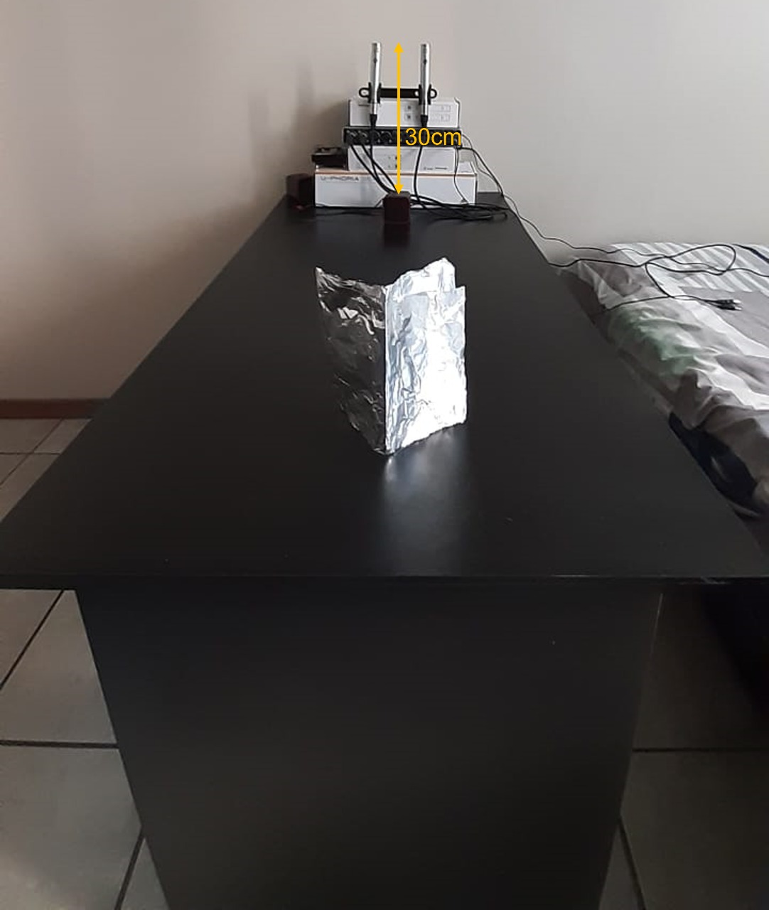
EDIT: Not realizing that the environment is also very important, I have now attached pictures of my physical setup.

EDIT: There are some changes with the help from you guys and some more research! Firstly, my microphone and speaker setup was off as the best configuration is as follows since the peak is where sound is best captured:

Secondly, Peter K. conveyed some insightful knowledge on chirps to me and it is yet to be implemented. I have also realised that enveloping the chirp removes energy from each side so tests will have to be re-run.

Thirdly, I have changed my equation for the matched filter to be:

def matchedFilter(signalRec, signalWinHann, FFT_side):
    print("Applying Matched Filter...\n")
    signalMF3 = np.abs(np.convolve(hilbert(signalRec), np.conj(np.flipud(hilbert(signalWinHann)))))
    padding = np.zeros(len(signalRec)//2)
    print("Maximum peak at: " + str(signalMF3.argmax()))
    plt.semilogy(signalMF3, color='blue', lw=2)
    plt.xlim(0, 2000)
    plt.xlabel('Range (m)')
    plt.ylabel('Amplitude')
    plt.show()
    aSignal = hilbert(np.abs(signalMF3))
    envelope = np.abs(aSignal)
    norm = envelope*44100 / (sum(envelope))
    print("\nMatched Filter Applied.\n")

    return norm

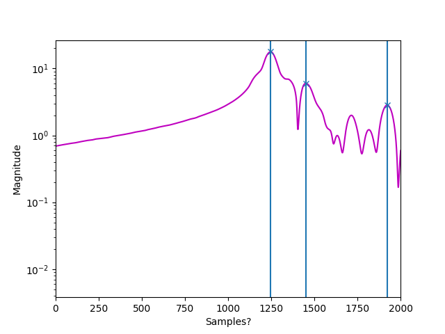
After the following run of the same chirp described above applied to my signal, I receive the following graph:

It is seen, after scaling, that I am correctly detecting the objects with an error of around ~5cm at various distances. The graph above was for detection of a ~6cm Cylindrical object placed 75cm from the transmission source.

Fourthly, Matched Filtering is considered "Optimum" in filtering noise from a signal thus no other filters like a LPF or BPF was required in order to correctly get the right results.

My next step in object detection is to determine the Angle of the reflected pulses using the inputs from the two microphones using a method called multi-lateration of 1 transmitter and 2 receivers. I hope to receive this well as it is necessary to get the correct bearing of the object.

Should I be splitting the channels coming in from each signal? I am currently unsure?

Thank you guys so much for your help thus far! I hope that this post may help someone someday as much as you guys are helping me !

Answer 1

I'm not sure it's your only issue, but I don't think you've "chirped" enough (the maximum and minimum frequencies of your chirp are not far enough apart).

Because of this, you get:

where the top curve is the chirp, the middle curve is the FFT and the bottom curve is the matched filter output.

I've set

f1 = 4000;
f2 = 4400;

in the matlab code below to do this.

If, instead, you go with:

f1 = 4000;
f2 = 12000;

then I get:

which shows a much cleaner pulse at the output of the matched filter.

Have a read through this page for the details.

---

Matlab code below

T = 1000;
fs = 44100;
t = [0:T-1]/fs;

f1 = 4000;
f2 = 12000;

x = chirp(t,f1,t(T) , f2);
xg = x.*exp(-0.005*abs([0:T-1]-(T-1)/2).^2/T);
figure(1);
clf;
subplot(311);
plot(x);
hold on;
plot(xg,'r');
subplot(312);
plot(abs(fft(x)));
hold on;
plot(abs(fft(xg)),'r');
subplot (313);
plot(xcorr(x,x));
hold on;
plot(xcorr(xg,xg),'r');
axis([950 1050 -400 600])