Given a sinusoidal signal in white noise, how can one efficiently determine its frequency?
-
2$\begingroup$ If you're certain it's sinusoidal and there are no other components to it other than broadbanded.noise, and you know nothing else about it, in advance, then window a segment of the input, run that into an FFT, and find where the maximum magnitude is. $\endgroup$– robert bristow-johnsonCommented Aug 8, 2021 at 11:47
-
3$\begingroup$ What do you have? Samples? What do you know? Is this a Sine signal with noise? How long is the sampling interval? $\endgroup$– MarkCommented Aug 8, 2021 at 12:47
-
3$\begingroup$ Are we computationally limited? $\endgroup$– MarkCommented Aug 8, 2021 at 12:49
-
3$\begingroup$ Please state requirements. Rough SNR (-100 dB, -50 dB, -10 dB, etc.). Class of noise, e.g. white, pink, spikey, harmonic, etc. "Efficient" in terms of what? Time to estimation, CPU consumption, Memory consumption ? $\endgroup$– HilmarCommented Aug 8, 2021 at 14:37
-
4$\begingroup$ This question is far too broad. Please edit your question to define what you mean by "efficiently", what are the characteristics of the signal (distortion, amplitude, noise, presence and amplitude of interfering signals), how long the observation interval is, and how accurately frequency needs to be determined. And, of course, anything I forgot to include. These factors all determine the most "efficient" way to determine a signal's frequency. $\endgroup$– TimWescottCommented Aug 8, 2021 at 20:06
9 Answers
I assume the model to be:
$$ x \left[ n \right] = \sin \left[ 2 \pi \frac{f}{ {f}_{s} } n + \phi \right] + w \left[ n \right] $$
Where $ w \left[ n \right] $ is white noise uncorrelated with the signal itself.
The obvious method here would be using DFT as the Maximum Likelihood Estimator of such case. It will probably be able to generate the best results in low SNR.
In High SNR I would use the method in Steven Kay - A Fast and Accurate Single Frequency Estimator (Alternative Source).
There are 2 methods given there.
The simplest one (Eq. 17 in the paper) is basically:
estFreq = 0;
for ii = 1:(numSamples - 1)
    estFreq = estFreq + angle(vX(ii)' * vX(ii + 1));
end

estFreq = estFreq / (2 * pi * (numSamples - 1));
estFreq = samplingFreq * estFreq; %<! Moving from normalized frequency to absolute frequency
The intuition is very simple, basically estimating the slope of the instant phase.
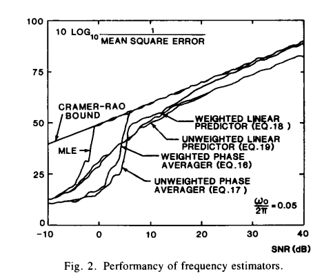
As can see from the paper, they achieve very good results in many real world case:
In Depth Analysis
The algorithm above, (Equation 17 in the paper) becomes, basically, zero crossing counting for real signal. It integrates many crossings (Assuming having many of those) hence better than just one. The issue is the assumption the phase is known and is 0.
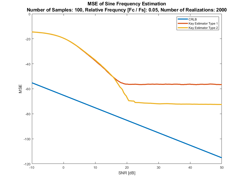
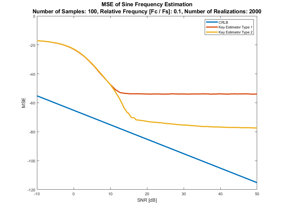
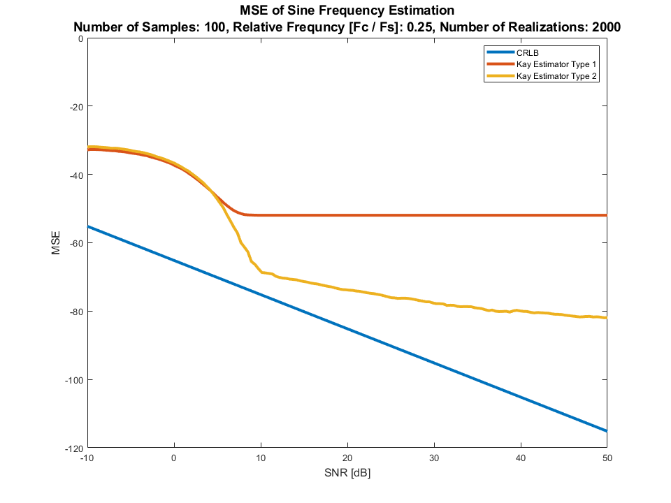
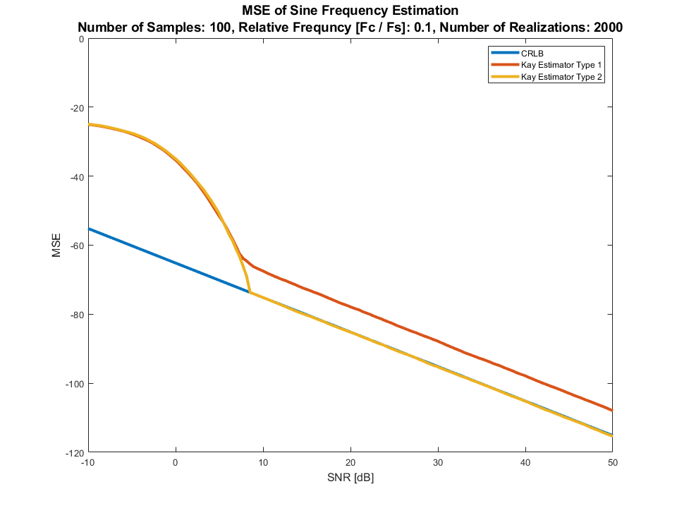
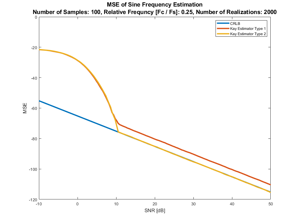
This is an example of its performance compared to the CRLB of estimating the frequency of a sine signal without any knowledge on its amplitude (Won't make a difference even if it is known) or phase:
The Kay Estimator Type 1 is the estimator from Eq. 17. The Kay Estimator Type 2 is Eq. 16 (With better weighing).
As expected, when the phase isn't known the performance aren't matching the CRLB. But real world performance are pretty good (Standard deviation of ~0.03 [Hz] at 5 [dB] SNR, Since it is normalized frequency one can thing of ~3%).
The above is done for 3 different relative frequencies yes for a random phase per realization.
We need specific frequency so in 2000 realization the curve will be smooth enough (For random frequency we'll probably need something in the range for 2 orders of magnitude more realizations).
Can we do better?
Yes!
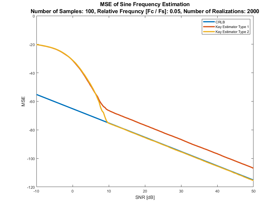
If we have a real signal (Sine / Cosine) all needed is to apply Hilbert Transform (Actually build the analytic signal as in MATLAB's hilbert()).
Sometimes, this analytic signal is what we have to begin with (See remarks).
Then, we get:
Well, this is it. We have something which match the CRLB for SNR of 9 [dB] and above and works pretty well even below it.
In summary:
- If you want good results (but not the best) with very simple algorithm, take the algorithm above and apply it directly on the real data. It is simple and work good enough. It assumes you have few cycles of the data.
- If you want a CRLB like results (As good as it gets) for SNR of
~9 [dB]apply Hilbert transform before calling the algorithm. It will add complexity but results will be as good as it gets without DFT analysis.
Remark 001: Pay attention that neither of the algorithms will work for other models. Namely with more than a single tone or something like that.
Remark 002: If those algorithm are used in the context of RF (RADAR, Communication, EW, SIGINT, etc...), then the Analytic Signal is "free".
-
1$\begingroup$ This is great. Specifically the intuition behind it. $\endgroup$– MarkCommented Aug 9, 2021 at 11:17
-
1$\begingroup$ This is cool. The tradeoff is being able to operate at lower SNR with MLE but computation time takes longer, or have a quicker computation time but require a higher SNR $\endgroup$– EngineerCommented Aug 9, 2021 at 13:11
-
1$\begingroup$ @Neil_UK, This will work: citeseerx.ist.psu.edu/viewdoc/…. $\endgroup$– RoyiCommented Aug 9, 2021 at 14:05
-
1$\begingroup$ @Royi, please consider editing the second bullet in the summary... $\endgroup$ Commented May 26, 2022 at 18:42
-
1$\begingroup$ @Royi, It will add complexity but results will be as good as it gets without DFT analysis. $\endgroup$ Commented May 26, 2022 at 18:45
A common way to do this is to take the FFT of the input signal. Since the frequency might not be right at a FFT bin, usually a second step of interpolation is done after choosing the initial peak. A couple reasons why this is commonly done is that it is the maximum likelihood solution for the AWGN case and no matter what platform you are implementing on there is likely an optimized FFT code out there for you to use. In terms of efficiency, you'd be looking at $\mathcal{O}(n\text{log}_2n)$ operations, where the heavy computational step is in taking the FFT.
If you have a low-noise and well-sampled signal, a quick way to estimate it is to find $\sqrt{-f''(t)/f(t)}$. For a signal $$f(t)=A \sin(\omega t+\phi)$$ the second derivative is $$-A \omega^2 \sin(\omega t+\phi)$$ which is $-\omega^2$ times the original. This is useful if you want a quick response and only have part of a cycle, so no zero-crossings. But obviously it depends on being able to get an accurate second derivative numerically.
-
$\begingroup$ It depends in particular also on being able to compute the second derivative. Whilst it's easy to estimate that with finite differences, this is highly susceptible to noise. $\endgroup$ Commented Aug 8, 2021 at 23:39
This depends on the precision needed.
If it's a pure sine wave that's noise free, you can get a very quick estimate by measuring the difference between two zero crossings.
The tricky part is that most sine wave frequencies are not integer dividers of the sample rate, so the actual zero-crossing falls between two samples and there is some inherent measurement error in this method.
The easiest way to deal with this is simply to keep measuring and averaging the results over time.
A more effective and quicker method is to estimate the exact location of the zero crossing through linear interpolation. This works quite well since a sine wave can be approximated as a line around it's zero crossing, i.e. $sin(x) \approx x, x \approx 0$. This will give you a very good estimate in a single measurement, but only if there is very little or no noise.
If things get noisy, if there are harmonics, or if there is drift, a better option is to use phase or delay locked loop to track the frequency.
Another thing to note is that you are can only measure the frequency in relation to your sample clock. Most real world sample clocks are drifting as well (albeit only by very small amounts).
If you want to go super quick you can use the relationship
$$y[n] = 2\cos(\omega) \cdot y[n-1] -y[n-2]$$
...which you can solve for $cos(\omega)$ using only three consecutive samples of the sine wave.
$$ \cos(\omega) = \frac{y[n]+y[n-2]}{2y[n-1]} $$
This method is numerically "fragile" and even a tiny amount of noise can lead to large errors
-
1$\begingroup$ I don't understand why this answer was voted down. It's a totally valid approach IMHO... $\endgroup$ Commented Aug 8, 2021 at 14:36
-
1$\begingroup$ Will it ever work in real life? It seems it won't. Could you compare it to other methods? $\endgroup$– MarkCommented Aug 9, 2021 at 11:18
-
3$\begingroup$ I think your equation about $ \cos \left( \omega \right) $ is wrong. The denominator should be $ 2 y \left[ n - 1 \right] $. $\endgroup$– RoyiCommented Aug 11, 2021 at 7:45
-
$\begingroup$ @Mark Better frequency calculations can be obtained by averaging many of these calculations with mean, median, or some more exotic statistical means. How much of a dataset is needed for averaging to the desired precision will be limited by the Shannon-Hartley theorem. That's a hard limit. It might be possible to prune the data better by weighting the values with a bell curve centered around the expected frequency. $\endgroup$ Commented Mar 28 at 20:33
I wasn't going to answer this, since the question is stale. But I'm a little bit dissatisfied with Royi's answer and with the Kay algorithm as presented.
The Kay method is, at first glance, simply using the analytic signal, which is what comes out of MATLAB's hilbert() operator, and then deriving the phase increment out of that to get away from the phase wrapping problem. This phase increment is your instantaneous frequency, and if your sinusoid has mostly unchanging frequency (a true sinusoid has constant frequency), then the instantaneous frequency should be mostly DC and low-pass filtering will attenuate noise and increase the resolution and accuracy of the estimated frequency. This is a very old idea and even predates the Kay paper. I think the Rife and Boorstin paper that Kay cited might be the earliest reference. I dunno. It's in O&S or Rabiner and Schafer or Papoulis or some old text.
First, let's start with noise-free input. Let's also assume that the input is DC free (run it through a DC-blocking HPF if you need to).
$$\begin{align} x[n] &= A \cos(\omega_0 n + \theta) \qquad\qquad\qquad A>0, \quad 0 < \omega_0 < \pi \\ \\ &= \tfrac{A}{2}\left(e^{j(\omega_0 n + \theta)} + e^{-j(\omega_0 n + \theta)}\right) \\ \end{align}$$
We compute the Hilbert transform
$$\begin{align} \hat{x}[n] &= \mathscr{H}\big\{ x[n] \big\} \\ \\ &\approx \sum\limits_{i=-L}^{+L} \frac{1-(-1)^i}{\pi \ i} w[i] \ x[n-i] \end{align}$$
and then analytic signal:
$$ x_\mathrm{a}[n] \triangleq x[n] + j \hat{x}[n] $$
$L$ should be a large, positive, and odd integer. The Hilbert transformer is an FIR filter with $2L+1$ taps (of which $L$ interlaced taps have zero coefficients and need not be computed) and $w[n]$ is a good window function. If it were a Hamming Window, it would be:
$$ w[n] = \begin{cases} 0.54 \ + \ 0.46 \cdot \cos\left(\pi \frac{n}{L} \right) \qquad & |n| \le L \\ 0 & |n| > L \\ \end{cases}$$
If it were a Kaiser window it would be
$$ w[n] = \begin{cases} \frac{1}{I_0(\beta)} \, I_0\left(\beta \sqrt{1 - \left(\frac{n}{L}\right)^2 } \right) \qquad & |n| \le L \\ 0 & |n| > L \\ \end{cases}$$
where
$$ I_0(u) \triangleq \sum\limits_{k=0}^{\infty} \frac{(-1)^k \big( \tfrac{u}{2} \big)^{2k}}{(k!)^2} $$
is the zeroth-order Bessel function of the first kind. With the Kaiser window, knowing the length $L$ (like $L$ might be 31 samples, or 63 if you want it really good) you can choose $\beta$ to tradeoff between the ripple and transition bandwidth around DC of the Hilbert transformer FIR. A good value of $\beta$ is 6 or 7, to get you about -63 dB or -72 dB of ripple around DC.
This Hilbert transformer is not causal but this implementation is FIR and a delay of $L$ samples will make it causal and "realizable" for real-time operation. So instead of $x_\mathrm{a}[n]$, you're really going to have $x_\mathrm{a}[n-L]$, but that delay should not be a problem if $L$ is reasonably small (not in the thousands). This means, when constructing the analytic function that, since $\hat{x}[n]$ is delayed by $L$ samples, so also must the input $x[n]$, to do this correctly. For simplicity, I will not depict that delay until maybe the very end.
Now after applying the Hilbert transform and computing the analytic function, only the positive frequency component survives (and gets doubled):
$$\begin{align} x_\mathrm{a}[n] &= x[n] + j \hat{x}[n] \\ \\ &= A \, e^{j(\omega_0 n + \theta)} \\ \end{align}$$
To get the phase increment, we can compute the $\log(\cdot)$ (which involves the $\arg\{\cdot\}$) and subtract the exponents of two adjacent samples of $x_\mathrm{a}[n]$, but that will require phase unwrapping (otherwise you will get a spurious spikes of $-2 \pi$ added to some phase increments). A better way to get the phase increment is simply to divide the two values and get the phase increment from that:
$$\begin{align} \frac{x_\mathrm{a}[n]}{x_\mathrm{a}[n-1]} &= \frac{A e^{j(\omega_0 n + \theta)}}{A e^{j(\omega_0 (n-1) + \theta)}} \\ \\ &= e^{j \omega_0} \end{align}$$
See how the amplitude $A$ and constant angle offset $\theta$ get killed off?
$$\begin{align} \omega_0[n] &= \arg \left\{ \frac{x_\mathrm{a}[n]}{x_\mathrm{a}[n-1]} \right\} \\ \\ &= \arg \left\{ \frac{x_\mathrm{a}[n] \, (x_\mathrm{a}[n-1])^*}{x_\mathrm{a}[n-1] \, (x_\mathrm{a}[n-1])^*} \right\} \qquad \qquad (\cdot)^* \text{ is complex conjugate}\\ \\ &= \arg \left\{ \frac{x_\mathrm{a}[n] \, (x_\mathrm{a}[n-1])^*}{\big| x_\mathrm{a}[n-1] \big|^2} \right\} \\ \\ &= \arg \Big\{ x_\mathrm{a}[n] \, (x_\mathrm{a}[n-1])^* \Big\} \\ \\ &= \arg \Big\{ (x[n] + j \hat{x}[n]) \, (x[n-1] - j \hat{x}[n-1]) \Big\} \\ \\ &= \arg \Big\{ (x[n]x[n-1] + \hat{x}[n]\hat{x}[n-1]) \, + \, j \big(\hat{x}[n]x[n-1] - x[n]\hat{x}[n-1] \big) \Big\} \\ \end{align}$$
Now I am showing the instantaneous frequency $\omega_0$ as a function of time $n$, in case the phase increment is not constant. And we know that $0 < \omega_0[n] < \pi$ so we have a single half-plane for the $\arg\{\cdot \}$ function. We'll use the second line.
$$ \arg \big\{ u+jv \big\} = \begin{cases} \arctan\left(\frac{v}{u}\right) &\text{if } u > 0, \\ \frac{\pi}{2} - \arctan\left(\frac{u}{v}\right) &\text{if } v > 0, \\ -\frac{\pi}{2} - \arctan\left(\frac{u}{v}\right) &\text{if } v < 0, \\ \arctan\left(\frac{v}{u}\right) \pm \pi &\text{if } u < 0, \\ \text{undefined} &\text{if } u = 0 \text{ and } v = 0 \end{cases} $$
So, I think, after computing the Hilbert transform $\hat{x}[n]$, we get for instantaneous frequency:
$$ \boxed{ \omega_0[n] = \tfrac{\pi}{2} - \arctan\left(\frac{x[n]x[n-1] + \hat{x}[n]\hat{x}[n-1]}{\hat{x}[n]x[n-1] - x[n]\hat{x}[n-1]}\right) } $$
So that's how you get the instantaneous frequency of a single real sinusoid $x[n]$ in a noise-free environment. Note that all of this is really delayed by $L$ samples because the Hilbert transformer is delayed by that.
So I'm gonna rob a Wikipedia graphic and make lotsa assumptions that I think are prudent. We'll say that $q[n]$ is additive Nyquist-bandlimited white Gaussian noise with zero mean and $\overline{q^2[n]}$ variance.
So it's added:
$$\begin{align} x[n] &= A \cos(\omega_0 n + \theta) + q[n] \qquad\qquad\qquad A>0, \quad 0 < \omega_0 < \pi \\ \\ &= \tfrac{A}{2}\left(e^{j(\omega_0 n + \theta)} + e^{-j(\omega_0 n + \theta)}\right) + q[n] \\ \end{align}$$
The Hilbert transform is:
$$ \hat{x}[n] = A \sin(\omega_0 n + \theta) + \hat{q}[n] $$
where $\hat{q}[n] = \mathscr{H}\big\{ q[n] \big\}$.
The analytic signal is
$$\begin{align} x_\mathrm{a}[n] &= x[n] + j \hat{x}[n] \\ \\ &= A \, e^{j(\omega_0 n + \theta)} + q[n] + j \hat{q}[n] \\ \end{align}$$
While $q[n]$ and $\hat{q}[n]$ are certainly coupled, they're both still Gaussian and white and have virtually the same energy or variance because the Hilbert transformer has 0 dB gain for all frequencies except DC and Nyquist.
$$ \overline{\hat{q}^2[n]} = \overline{q^2[n]}$$
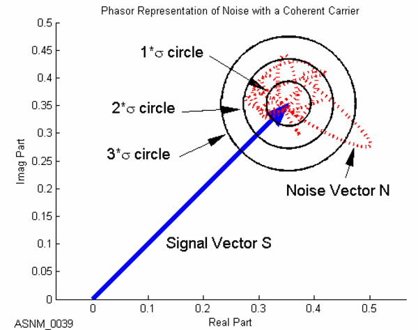
So, I think it's gonna look a bit like this figure
and, assuming a decent S/N ratio,
$$\begin{align} x_\mathrm{a}[n] &= x[n] + j \hat{x}[n] \\ \\ &= A \, e^{j(\omega_0 n + \theta)} + q[n] + j \hat{q}[n] \\ \\ &= A \, e^{j(\omega_0 n + \theta)} \left(1 + \tfrac{1}{A}e^{-j(\omega_0 n + \theta)}\big(q[n] + j \hat{q}[n]\big) \right) \\ \\ &= A \, e^{j(\omega_0 n + \theta)} \big(1 + \epsilon[n] \big) \\ \\ &\approx A \, e^{j(\omega_0 n + \theta)} e^{\epsilon[n]} \\ \\ &= A \, e^{j(\omega_0 n + \theta) + \epsilon[n]} \\ \end{align} $$
$\epsilon[n]$ is complex...
$$\begin{align} \epsilon[n] &= \tfrac{1}{A}e^{-j(\omega_0 n + \theta)}\big(q[n] + j \hat{q}[n]\big) \\ \\ &= \tfrac{1}{A}\big(\cos(\omega_0 n+\theta)q[n]+\sin(\omega_0 n+\theta)\hat{q}[n]\big) \\ & \qquad \qquad + j \tfrac{1}{A}\big(-\sin(\omega_0 n+\theta)q[n]+\cos(\omega_0 n+\theta)\hat{q}[n]\big) \\ \end{align}$$
... with the magnitude square having mean
$$\begin{align} \overline{|\epsilon[n]|^2} &= \frac{1}{A^2}\left(\overline{q^2[n]}+\overline{\hat{q}^2[n]}\right) \\ \\ &= \frac{2 \, \overline{q^2[n]}}{A^2} \\ \end{align}$$
And the variance of either the real part or the imaginary part:
$$\begin{align} \overline{\big(\Re e \{\epsilon[n]\}\big)^2} &= \tfrac12 \overline{|\epsilon[n]|^2} \\ \\ \\\overline{\big(\Im m \{\epsilon[n]\}\big)^2} &= \tfrac12 \overline{\big|e[n]\big|^2} \\ \\ &= \frac{\overline{q^2[n]}}{A^2} \\ \end{align}$$
It is the imaginary part, $$\Im m \{\epsilon[n]\}=\tfrac{1}{A}\big(-\sin(\omega_0 n+\theta)q[n]+\cos(\omega_0 n+\theta)\hat{q}[n]\big)$$, that is the additive error to the increasing phase of the sinusoid.
So now let's re-examine this with this Gaussian error added.
$$\begin{align} \frac{x_\mathrm{a}[n]}{x_\mathrm{a}[n-1]} &= \frac{A e^{j(\omega_0 n + \theta) + \epsilon[n]}}{A e^{j(\omega_0 (n-1) + \theta) + \epsilon[n-1]}} \\ \\ &= e^{j \omega_0 + \epsilon[n] - \epsilon[n-1]} \\ \\ &= e^{ \Re e \{\epsilon[n]\} - \Re e \{\epsilon[n-1]\} } \ e^{j (\omega_0 + \Im m \{\epsilon[n]\} - \Im m \{\epsilon[n-1]\}) } \\ \end{align}$$
So now this looks like:
$$ \arg \left\{ \frac{x_\mathrm{a}[n]}{x_\mathrm{a}[n-1]} \right\} = \omega_0 + \Im m \{\epsilon[n]\} - \Im m \{\epsilon[n-1]\} $$
or
$$ \omega_0[n] = \arg \left\{ \frac{x_\mathrm{a}[n]}{x_\mathrm{a}[n-1]} \right\} - \Im m \big\{\epsilon[n]\big\} + \Im m \big\{ \epsilon[n-1]\big\} $$
Now, this is what Royi and others are not going to like: I will make the further assumption that the two random values $\Im m \big\{\epsilon[n]\big\}$ and $\Im m \big\{\epsilon[n-1]\big\}$ are essentially not correlated to each other, so that their variances add and, for this single value of instantaneous frequency, $\omega_0[n]$, the added error has variance of $\frac{2 \, \overline{q^2[n]}}{A^2}$. That might be a little iffy but, even if they were perfectly correlated, the variance of the added error cannot exceed $\frac{4 \, \overline{q^2[n]}}{A^2}$.
But, because this error is really added to the phase (and not to the frequency), averaging really helps. Suppose we have a moving average filter working on the estimate of $\omega_0[n]$:
$$\begin{align} \overline{\Omega_M}[n] &= \frac{1}{M} \sum\limits_{m=0}^{M-1} \arg \left\{ \frac{x_\mathrm{a}[n-m]}{x_\mathrm{a}[n-m-1]} \right\} \\ \\ &= \frac{1}{M} \arg \left\{ \frac{x_\mathrm{a}[n]}{x_\mathrm{a}[n-1]} \times \frac{x_\mathrm{a}[n-1]}{x_\mathrm{a}[n-2]} \times ... \frac{x_\mathrm{a}[n-(M-1)]}{x_\mathrm{a}[n-M]} \right\} \\ \\ &= \frac{1}{M} \arg \left\{ \frac{x_\mathrm{a}[n]}{x_\mathrm{a}[n-M]} \right\} \\ \\ &= \frac{1}{M} \sum\limits_{m=0}^{M-1} \omega_0[n-m] + \Im m \big\{\epsilon[n-m]\big\} - \Im m \big\{ \epsilon[n-m-1] \big\} \\ \\ &= \frac{1}{M} \sum\limits_{m=0}^{M-1} \omega_0[n-m] + \frac{1}{M} \sum\limits_{m=0}^{M-1} \Im m \big\{\epsilon[n-m]\big\} - \Im m \big\{ \epsilon[n-m-1] \big\} \\ \\ &= \overline{\omega_0[n]} + \frac{1}{M} \sum\limits_{m=0}^{M-1} \Im m \big\{\epsilon[n-m]\big\} - \Im m \big\{ \epsilon[n-m-1] \big\} \\ \\ &= \overline{\omega_0[n]} + \frac{1}{M} \Big( \Im m \big\{\epsilon[n]\big\} - \Im m \big\{ \epsilon[n-M] \big\} \Big) \\ \\ &= \overline{\omega_0[n]} + \xi[n] \\ \end{align}$$
What's happening here is that the phase error of sample $n-m-1$ gets cancelled by the phase error of sample $n-m$ and only the two phase errors at the endpoints remain. So the instantaneous frequency gets to team up with a factor of $M$, but the phase error cannot.
So the estimate of the sliding mean of instantaneous frequency is equal to the actual sliding mean of instantaneous frequency plus an error term with mean square that is
$$ \overline{\xi^2[n]} = \frac{2 \, \overline{q^2[n]}}{M^2 A^2} $$
or r.m.s. amplitude
$$ \sqrt{\overline{\xi^2[n]}} = \frac{\sqrt{2 \, \overline{q^2[n]}}}{M \, A} $$
Expressed in dB, this looks like:
$$ 10\log_{10}\left(\,\overline{\xi^2[n]}\,\right) = 10\log_{10}\left( \frac{\overline{q^2[n]}}{A^2/2} \right) - 20\log_{10}(M) $$
The first term right of $=$ is S/N ratio. If $M=$100 (which is in the examples of the other answers), then the last term is -40 dB. It's a curiosity to me how they (I dunno, Royi, Overlord, or Cedron) got the CRLB to be nearly twice the number of dB (looks like -65 dB when SNR=0). At first I thought they might have used "$20\log_{10}(\cdot)$" when they should have used $10\log_{10}(\cdot)$, but that doesn't explain why we agree on the slope of the line. I really do not understand where this 25 dB of extra performance comes from with the number of samples in the average $M=$100. I'm hoping someone can explain that.
I'm gonna leave it here and let it take some incoming critique and maybe modify it later. The method remains unchanged, it's just that this gives us an idea about how the added noise causes an added error to the frequency measurement with $M+1$ samples (and $2L$ additional samples, to compute the Hilbert transform).
So the bigger the amplitude of your sinusoid, $A$, the better. The smaller of the amplitude of your AWGN, $\sqrt{\overline{q^2[n]}}$, the better. And the more values of instantaneous frequency in the average, $M$, the better. This averaging is really low-pass filtering, and I believe that other LPF methods, like a 1st-order recursive (or "leaky integrator"), will work just as well.
-
$\begingroup$ Robert, the Kay algorithm doesn't require analytic signal. It is doing a decent work for signals as well. Anyhow, good analysis +1. $\endgroup$– RoyiCommented Jul 17, 2023 at 5:36
-
$\begingroup$ It's meant to be a "simple and effective method". The "analysis" was meant to justify the method. Now the method is defined, the question is how good it is when AWGN is added to $x[n]$. I haven't thunked up a symbol yet (since I am already using "$w[n]$" for the window applied to the Hilbert transformer impulse response). Then I gotta finagle the additive white noise to an error term in the exponent getting added to the phase. All that is analysis. $\endgroup$ Commented Jul 17, 2023 at 6:32
-
$\begingroup$ I liked the analysis. In the RF it is it is a little secret that when compute is sparse you can't beat Kay Type 2 (With some nice CRLB related weighing). You can see why, if the signal is analytic as in RF, it achieves the CRLB with complexity of
O(N). There is nothing more to ask as nothing practical is belowO(n)and certainly nothing can be better the CRLB (Unbiased). $\endgroup$– RoyiCommented Jul 17, 2023 at 7:21 -
$\begingroup$ Anyhow, it is always great to see more point of views. $\endgroup$– RoyiCommented Jul 17, 2023 at 7:24
-
1$\begingroup$ By the way, in the scenario of noise, it will make sense to average $ {w}_{0} \left[ n \right] $. The problem is the transformations are non linear and makes even white noise correlated as the result depends on few samples. So there is something more clever to do than a naïve averaging. Though it will require some math digging to extract the properties of the new distribution of noise. $\endgroup$– RoyiCommented Jul 17, 2023 at 7:29
As others have already mentioned in the comments, the question shows on research effort, is far too broad and needs clarification.
Depending on the requirements, the MUSIC (or ESPRIT) algorithm may be a suitable approach to efficiently find a high resolution frequency estimation. The algorithm is specifically intended for finding the frequency of sinusoids in additive noise by using a covariance approach.
Quoting the relevant passage of the linked Wikipedia article regarding efficiency:
In a detailed evaluation based on thousands of simulations, the Massachusetts Institute of Technology's Lincoln Laboratory concluded in 1998 that, among currently accepted high-resolution algorithms, MUSIC was the most promising and a leading candidate for further study and actual hardware implementation. Lincoln Laboratory - Performance Comparison of Array Processing Algorithms
Regarding its accuracy:
MUSIC outperforms simple methods such as picking peaks of DFT spectra in the presence of noise, when the number of components is known in advance, because it exploits knowledge of this number to ignore the noise in its final report.
Unlike DFT, it is able to estimate frequencies with accuracy higher than one sample, because its estimation function can be evaluated for any frequency, not just those of DFT bins.
-
1$\begingroup$ Those are very effective methods. Yet not easy to compute (Not computationally efficient). But it is nice to see more awareness to those here. +1. $\endgroup$– RoyiCommented Aug 11, 2021 at 7:43
Since @OverLordGoldDragon raised methods based on applying the DFT, I'd like to share another simple idea.
Given the DFT, if the number of bins is high enough (Zero padding if needed, choosing power of 2) the peak can be approximated by a quadratic formula.
So if we take one sample to the left of the peak and one to the right we can calculate the shift for the quadratic maximum using a simple calculation.
If we model the samples using the quadratic model:
p = ax^2 + bx + c
We can arbitrary do as following:
- Choose the current peak to have zero value.
- Decide the
xvalues are{-1, 0, 1}.
Which yields:
p1 = a - b
p2 = 0
p3 = a + b
Then we can easily calculate the maximum of the parabola using -b / 2a which will yield: (p1 - p3) / (2 * (p1 + p3)).
For the calculation p1, p2, p3 are the magnitude of the values around the peak of the DFT (p2 is the maximum).
The estimated frequency is basically (idxK - 1 + ((p1 - p3) / (2 * (p1 + p3)))) * (samplingFreq / numSamples). That's all.
So basically all we have is fft(), abs(), argmax() and extracting 3 values.
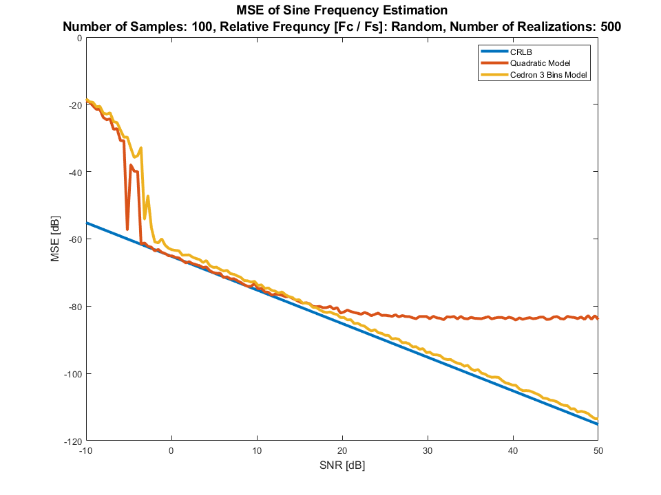
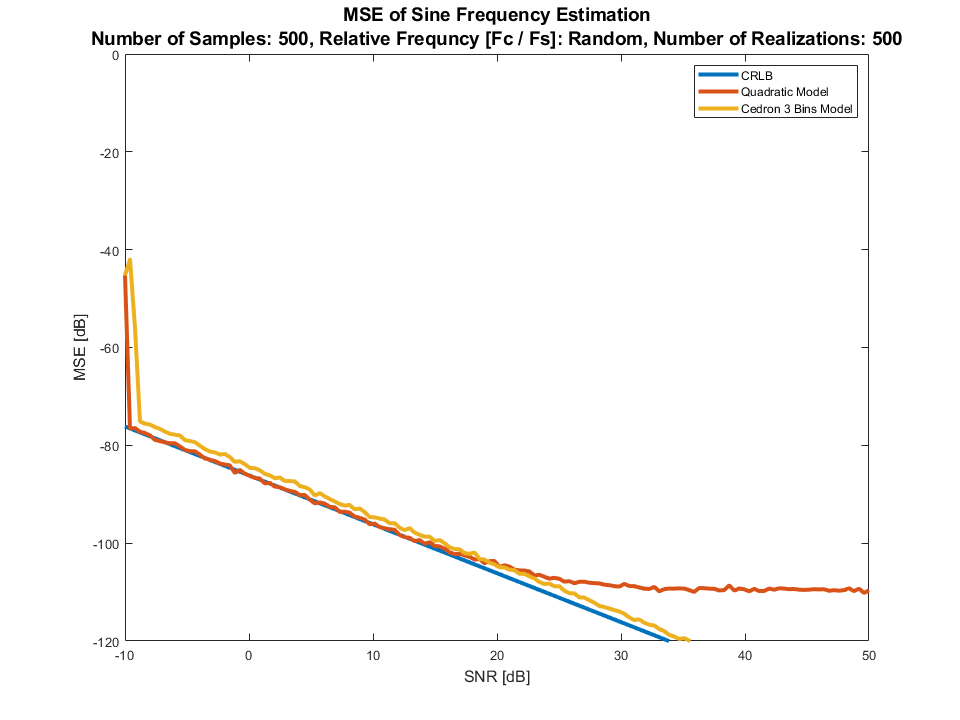
The results it yields (With fractional frequency):
The Cedron method is the 3 Bins accurate method in @OverLordGoldDragon post (The one in the graphs). In the experiment above the frequency is random over the realizations.
As long as the noise is the dominant cause of error the method is superior to Cedron's method.
When the SNR is very high, practically perfect signal, the bias in the model kicks in and leave the frequency error in the range of ~1e-5.
For any practical calculation having MSE of -75 [dB] is practically perfect.
I am not aware on anything simpler based on DFT beside zero padding to extreme.
In the case of longer signal, performance gets better.
This happens since the peak by the Dirichlet Kernel becomes better suited for quadratic approximation by less leakage (Better resolution).
From my experience, in real world use, if you do DFT to estimate the single tone, this is what you'd do.
Remark: If one want extra efficiently the close neighborhood of the peak can be calculated locally by the Goertzel Algorithm.
Remark: Nothing but appreciation for the work of Cedron Dawg.
Remark: Pay attention all those method doesn't work for mutli tone, Cedron's included. When saying Multi Tone in this context, it means where tones are close enough so one is within the main lobe of the other. Then looking for peaks is not relevant. There are tricks to over come this with simple methods, like peeling, (Though advanced Super Resolution is much better), but this is enough RADAR secrets for one day.
Summary
- Possible State of the Art by Cedron in compute-limited settings, as it beats Kay and many other methods
- In accuracy, Cedron is superior to Kay in nearly all settings, for both real and complex tones
- In speed, Cedron is superior to Kay in most or all cases, depending on version of Kay. In real case, if Kay uses Hilbert, Cedron is by far faster. Otherwise, in real, Kay is always faster (esp. large
N), but accuracy is very poor. In complex, Cedron is faster forN < ~100000, but they're close for mostN. For smallN, all are always very fast. See "Speed" & "Benchmarks" below. - Cedron handles multi-tones, Kay doesn't
- In noiseless case, Cedron exactly retrieves frequency, phase, and amplitude
- Royi's plots are cherrypicked. He is also a fraud.
Details
The Kay estimator described in Royi's answer, that matches CRLB, assumes a whole number of cycles of the sine, since it rests on the quality of the Hilbert transform. Performance degrades significantly for the general case.
The inverse problem solved from the sine DFT closed form solution is far more robust:
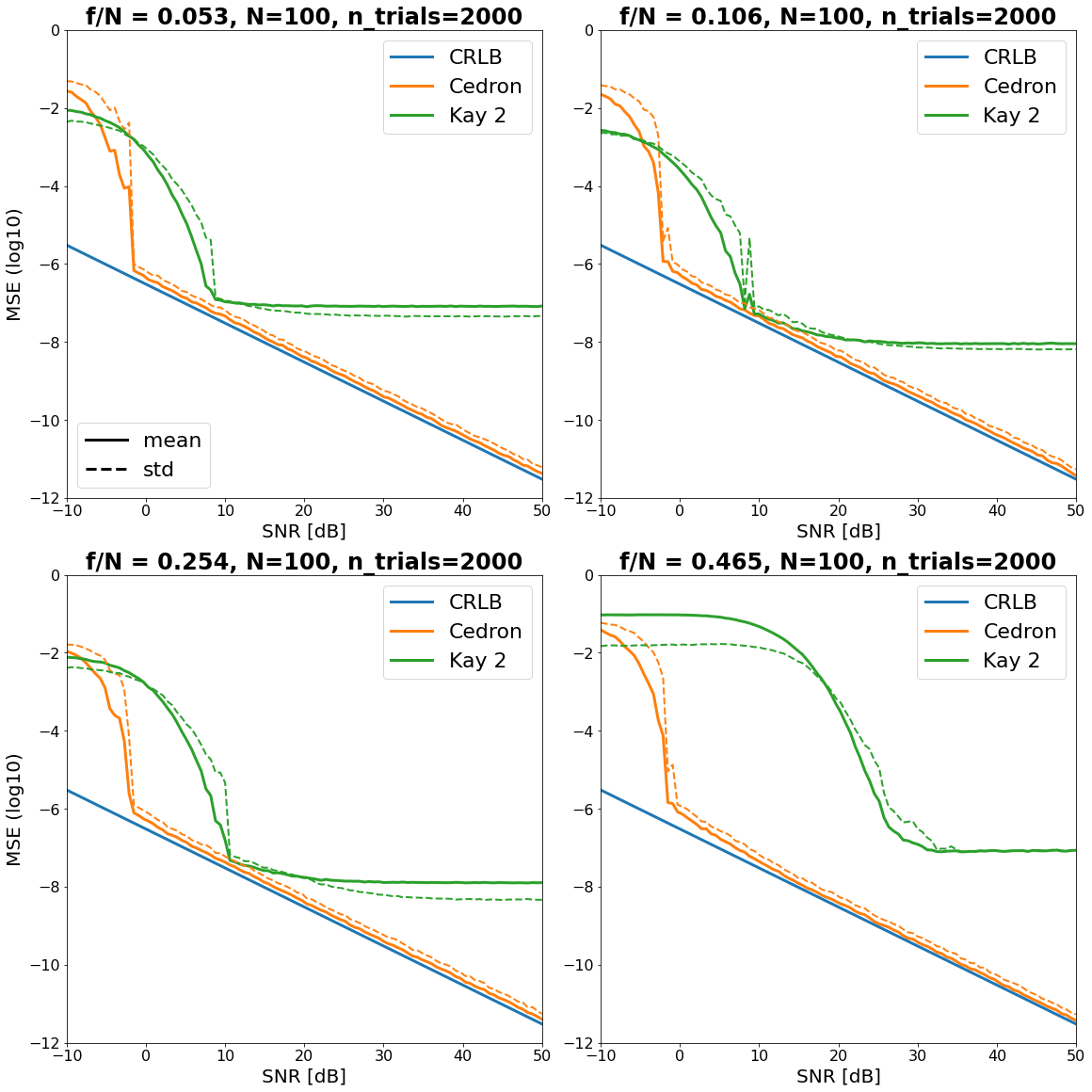
This is expected, since the DFT-based Hilbert is aliased for non-integer frequencies, and any Hilbert suffers edge effects, while Cedron's solution remains universally exact. Outside the few-sample regime, Kay 2 degrades in low SNR and improves in high SNR, while Cedron only improves:
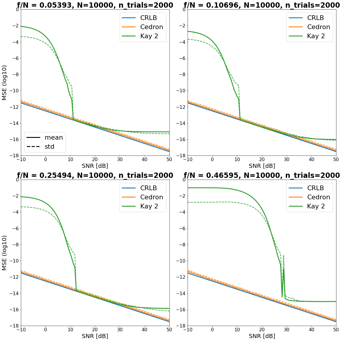
Hilbert performs excellent for all above cases with N=10000. Yet, Kay 2 is a time-domain estimator, and sample-to-sample variation is far greater with greater N, even if SNR is same, while the DFT remains robust. Hence, Kay 2's utility is limited relative to Cedron's. For integer or near-integer frequencies, Kay 2 retains a small edge over Cedron in high SNR - here's plots (it eventually ends since Cedron is exact in noiseless case).
For higher & lower SNR, both solutions retain their trends - here's plots. At db=-10, noise variance is already x10 greater than signal variance, and db=50 is x200,000 lesser, so the sweeps I've displayed cover most use cases.
Cedron's CRLB interval can be extended with Maximum Likelyhood Estimation and other methods, but they're compute-intensive.
Above plots worked with the model
$$ x[n] = \cos(2\pi (f/N)n + \phi_U) + w[n], $$
where $\phi_U$ is a random uniform realization over $[0, 2\pi]$, and $w[n]$ is White Gaussian Noise. It's same as Royi's formulation. Randomized phase since phase is unknown, and it doesn't make sense to favor any one $\phi$ when averaging performance over some $\text{n_trials}$.
Note, Royi's answer mistakenly states "results will be as good as it gets without DFT" (Hilbert uses two DFTs), which was also pointed out by a comment. This concerns both speed, and conceptual accuracy, since the DFT-Hilbert is inherently spectral.
Cedron's solution is described in his Improved Three Bin Exact Frequency Formula for a Pure Real Tone in a DFT. Kay 2's is in his A Fast and Accurate Single Frequency Estimator, and is overviewed in Royi's answer.
Speed
- Cedron, very fast: one
rfft, oneabs, oneargmax, and a few $O(1)$s. Theabsandargmaxnaively are $O(N)$, but this can be sped up for high SNR. Also don't need thesqrtinabs. - Kay 2, much slower:
arctan2alone is 3x slower thanrfftforN=100000, and pars it for smallN. Still very fast for smallN. In full: onerfft, oneifft(notirfft), an $O(N)$ zeros allocation (Hilbert), $O(N)$ complex conjugations, $O(N)$ complex-complex multiplications, $O(N)$ complex-real multiplications, $O(N)$ complex additions, $O(N)$ real divisions, $O(N)$ conditional sign handlings (atan2), and $O(N)$ arctangents. Note, conjugations and zeros are surprisingly slow; optimal coding can only remove the conjugation overhead. - Complex case: it's
fftfor Cedron, and Kay 2 dropsrfftandifft. It's now much closer, but Cedron is still faster unless $N$ is large (>$10^5$ or $10^6$ depending on device). See "Benchmarks (complex)" below.
Complex tones
In some applications, the sine is complex. We include negative frequencies, and linear sweep rather than random uniform to not repeat cases - results:
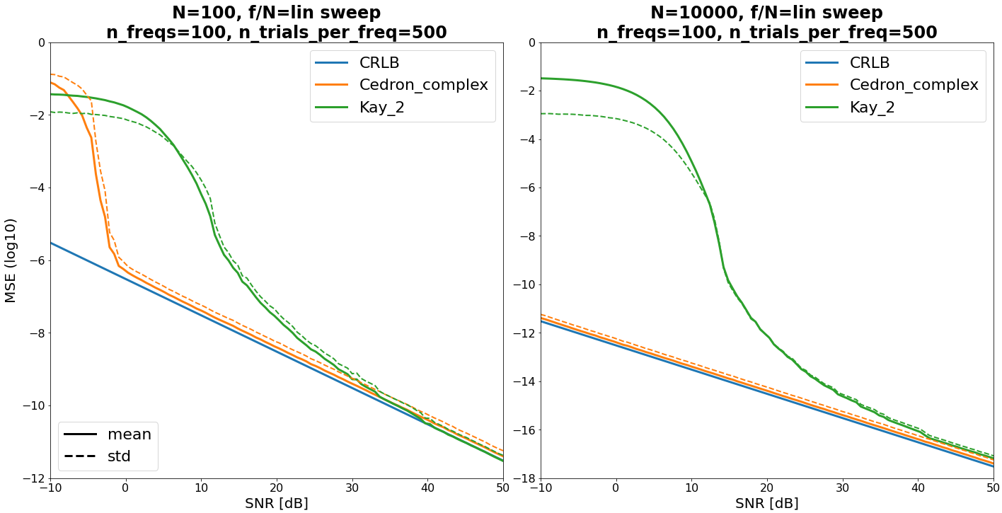
So, unless SNR is low or very high and samples are low, Cedron is always superior. In high SNR, when Cedron isn't superior, the gap is very small.
This uses Cedron 3-bin complex solution, and my implementation isn't ideal - Cedron describes steps to improve.
Note, Kay performance assumes an ideal complex tone, and degrades greatly if it's not (as shown in other sections' plots). In practice, complex tones may result from a Hilbert transformer. If tones are generated or otherwise excellent quality, then Kay works well in high SNR, as shown. In contrast, Cedron works well even if complex tones stem from poor quality DFT-Hilberts, via the real solution, as shown in other sections' plots.
Multi-tone estimation
Kay is limited to a single tone:
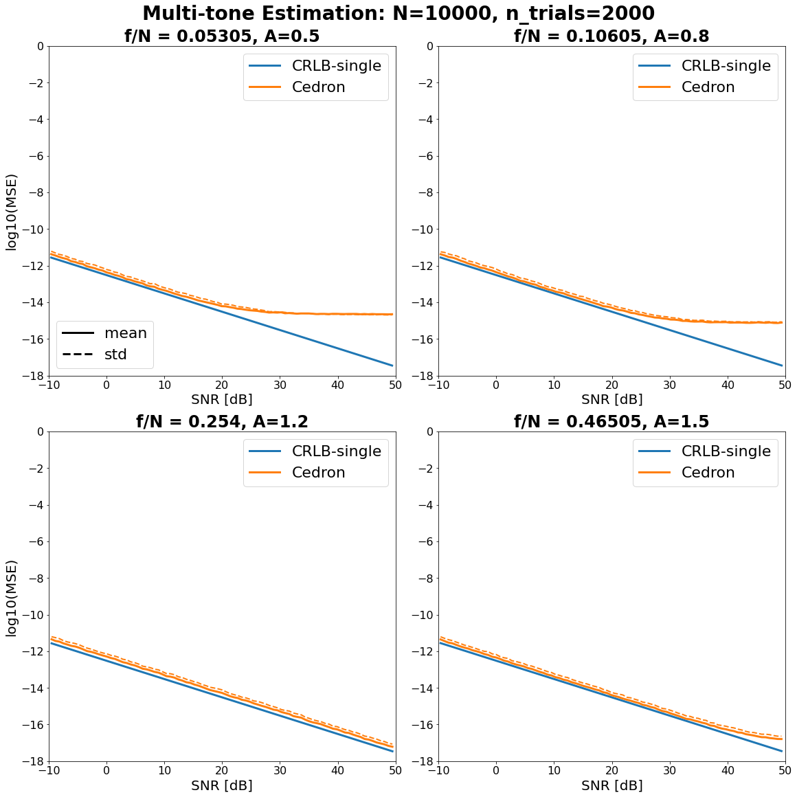
Four tones of different frequencies, amplitudes, and phases. Phases of each tone are independently random.
The true CRLB is greater than what's shown, and depends on tone spacing and count, and whether the count is known; I've shown CRLB for a single tone, but spaced out the tones greatly so it remains fair for the shown SNR range. For high SNR, tone interference dominates - this can be accounted for by estimating tone amplitudes and phases (which another of Cedron's solutions can do, exactly for single-tone noiseless) and eliminating them, which I haven't done here. Unknown count can also be handled, but common noise variance is amplitude-restricted.
Close tones can also be resolved, but not extremely close (leakage resolution) - here's plots; it's not CRLB, but it's still 1e-11 MSE. That's separate from the noiseless and iteratively eliminated case.
Note, f/N = 0.254 is integer frequency, and it performs better than the greatest amplitude. Also, the plots' x-axes are correct; I swept a greater range of SNR and discarded those outside of $[-10, 50]$ on per-tone basis, each tone's SNR computed as a single tone's (SNR is in-band).
A baseline is DFT argmax, here's plots, which I've not displayed since it may suggest the two methods are close when they aren't (elimination not implemented). Few samples also works, but limited without elimination - plots.
Extreme example
Is there a method that can recover a sine's frequency within 2e-5 MSE, for 1:1000 SNR (-30dB)? With just 2 seconds of typical audio, Cedron's method can, in one millisecond. The noising, visually:
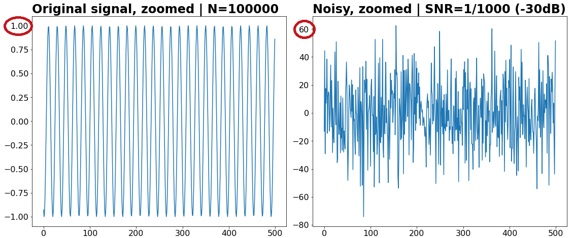
Kay 2 can only dream of this. Cedron's performance improves with greater N.
Noiseless case
Cedron is exact for all frequencies, also exactly recovering amplitude and phase. Interestingly, however, for integer frequencies, Kay retains a tiny edge. It is negligible, and the only possible explanation is numeric precision. Note, 200dB is $10^{-20}$, well-past float64 epsilon $10^{-16}$.
How's it work?
Cedron exploits the fact that white noise is uncorrelated with the sine; the inverse solution is in vector form, with many solutions, but only one subgroup that maximizes signal information:
The amount of the error can't be minimized by the appropriate selection of $\overrightarrow K$. However, the amount of signal information can be maximized. This is achieved by making $\overrightarrow K$ as close to the direction of $\overrightarrow A$ and $\overrightarrow B$ as possible. This requires projecting a vector onto the plane normal to $\overrightarrow C$ to find $\overrightarrow K$.
Another step is random variable variance equalization (eqs 18-20). Both are explained here.
The CRLB-matching interval rests upon the DFT; $f$ is found from DFT bins, which have highest SNR at signal's peak, and signal's DFT peak is eventually drowned out by noise. This is why the error suddenly jumps (and can be confirmed by plotting
argmax(abs(rfft(x))) errors). Maximum Likelyhood Estimation and other methods can hence extend said interval.
Benchmarks (complex)
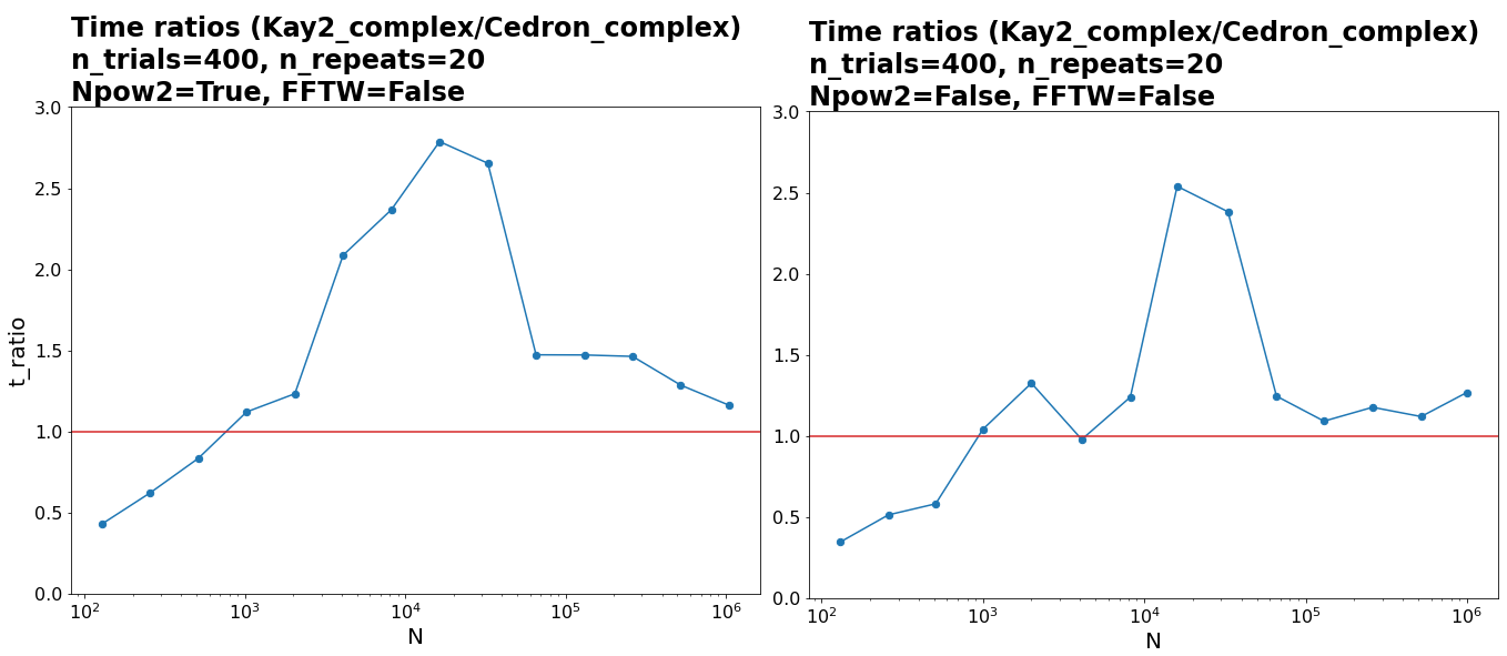
I implemented both algorithms in C, and tested their single-thread performance. On a powerful CPU:
On a much, much weaker CPU (still not microprocessor-grade), via repl-it (live code you can run online):
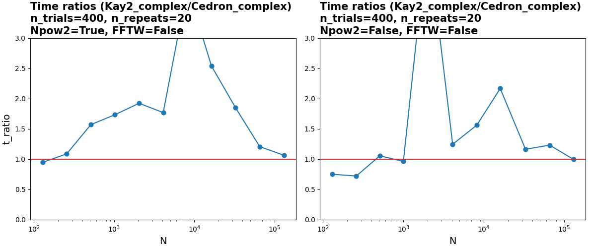
$O(N)$ means the full cost function is $c_0N + c_1$, where $c_1$ is miscellaneous CPU overhead. Cedron wins because $c_0$ for FFT ($c_0N\log(N)$) is much lower than it is for Kay 2. For particularly small $N$, Cedron can lose because of hardware optimizations (higher $c_1$) - caching, instructional vectorization, etc. Concerning n_trials and n_repeats, see 1 & 2.
FFT is just complex multiply-adds. Kay 2 is that plus arctangents, real ratios, and conditional sign-handling (atan2). Of course, for large enough $N$, Kay wins, since then there's simply much more multiply-adds in FFT.
FFTW can greatly speed up FFT, and wasn't used. It'd likely put Cedron above Kay everywhere. What's surprising is that Cedron is faster even for $N=10^6$ on the strong CPU. (Note, weak CPU tested only up to $N=10^5$, but likely Cedron would be slower there).
For most purposes, the two algorithms are basically equally fast, and are real-time up to a generous sampling rate. Yet, Cedron is far superior in accuracy. Note, all this analysis is for the complex case - for others, see "Summary" on top.
Lastly, I actually coded in Cython, which is often even faster than coding in plain C as it handles certain optimizations. The implems par ones coded in Numba, which is all about automated optimizations - given the algos' simplicity, a good sign they won't get much faster with expert optimizations.
Minimal code
import numpy as np

def est_f_cedron(x):
    # https://www.dsprelated.com/showarticle/773.php
    N = len(x)
    X = np.fft.rfft(x)
    k = np.argmax(abs(X[1:-1]))  # see full code regarding `1:-1`

    r = np.exp(-1j*2*np.pi/N)
    cosb = np.cos(2*np.pi/N * np.array([k-1, k, k+1]))

    num = -X[0]*cosb[0] + X[1]*(1 + r)*cosb[1] - X[2]*r*cosb[2]
    den = -X[0]         + X[1]*(1 + r)         - X[2]*r
    f = np.arccos(num/den).real / (2*np.pi)
    return f

N = 10000
f_frac = 0.12321
snr = -10

f = f_frac*N
phi = np.random.uniform(0, 2*np.pi)
sine = np.cos(2*np.pi*f*np.arange(N)/N + phi)
noise = np.random.randn(N) * np.sqrt(sine.var() / 10**(snr/10))
x = sine + noise

f_est = est_f_cedron(x)
print(f_frac, f_est, (f_frac - f_est)**2, sep='\n')
%timeit est_f_cedron(x)
0.12321
0.1231528108515302
3.2705987027014055e-09
66.7 µs ± 723 ns per loop (mean ± std. dev. of 7 runs, 10,000 loops each)
This is a simpler and somewhat weaker solution; the one demonstrated throughout the answer isn't much more complicated, see est_f_cedron_3bin in code linked below. Some implementations are speed-optimized (check optimized.py below).
Code
Available at Github.
To build _optimized.pyx, run python setup.py build_ext --inplace once cd'd into the directory. Included standalone, as a part of Cedron, is a fast complex abs_argmax.
-
$\begingroup$ Any cubic interpolation over the DFT get the ML performance. Nothing new here. The whole idea was without doing the DFT. $\endgroup$– RoyiCommented Jul 15, 2023 at 12:47
-
$\begingroup$ Also, The estimator works for any relation of the frequency and the number of samples. As I wrote, it requires few cycles, but certainly not integer multiplication I don't know what caused you assert this. Moreover, my analysis was with random phase. See i.imgur.com/H59Krwq.png. It is just requires much much more realizations with non integer frequencies. $\endgroup$– RoyiCommented Jul 15, 2023 at 13:13
-
$\begingroup$ Your complexity analysis is flawed. It is biased as you use Python hence working in a vectorized manner on arrays. Kay's methods are
O(n)with the constant being the calculation of the angle which for real signals is just the sign so nothing at all. Algorithms like that are usually used in the RF context where the analytic signal is "free". Then the cost staysO(n). $\endgroup$– RoyiCommented Jul 15, 2023 at 16:03 -
$\begingroup$ Usually, when those algorithms are used in real for RF, they are implemented on real time hardware, usually FPGA. If you care about the perfect performance, you do Maximum Likelihood with interpolation. In the context of simple, you can't beat the trick of Kay. For the noiseless case, you can do even simpler things, Like @Hilmar's answer. $\endgroup$– RoyiCommented Jul 15, 2023 at 16:09
-
$\begingroup$ Let's agree to disagree. $\endgroup$ Commented Jul 16, 2023 at 11:41
This extends my answer by responding to comments made about it.
if the number of bins is high enough
For N=100, I've only reproduced Royi's plots with Npad=2048, which is a massive caveat. And that was for one favorable frequency. Without cherrypicking, it's much worse. Since it's pointless to repeat a frequency, a linear sweep is a better test than randomized:
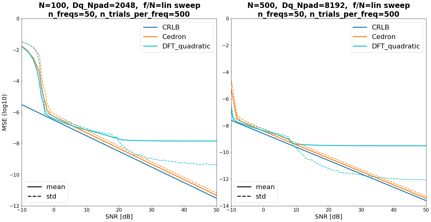
Fractional and near-integers included. DFT-quadratic's CRLB interval is greater only because of the longer FFT, and can be perfectly reproduced for Cedron. This includes the extended gap in the right plot, it's just a constant delay. If there's a smarter way to pick Npad, or something else Royi's done differently, Royi doesn't state it nor provide any code.
"Multitone" means multiple tones, nothing more. Kay 2 is incapable of handling it, and DFT-quadratic can't do better than DFT argmax:
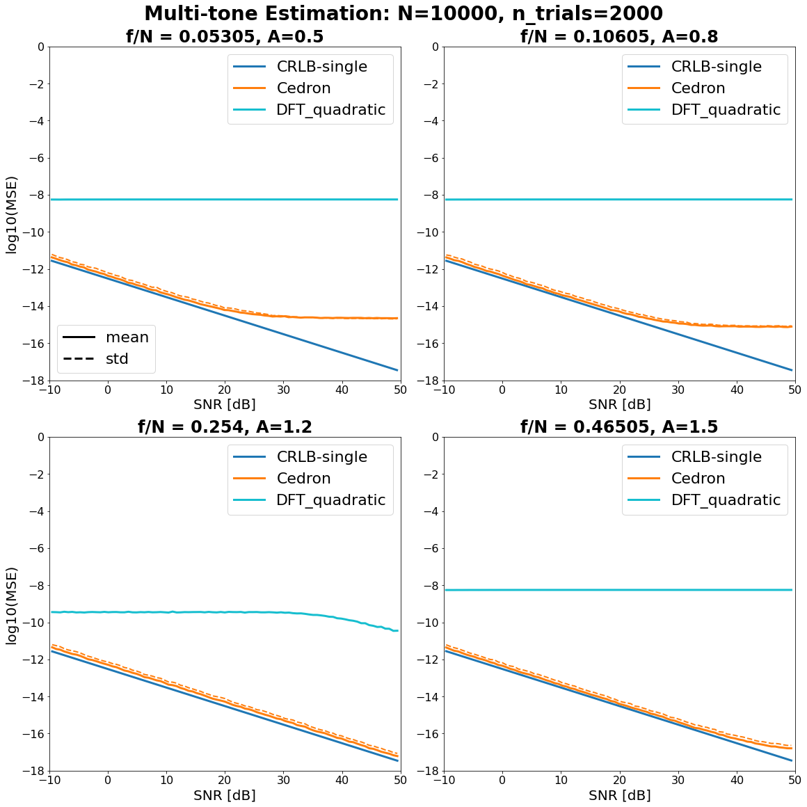
Again, Cedron performance can be improved with further steps. Without said steps, it also handles closely spaced tones, as I've shown in my other answer, but performance is limited. I didn't pad Dq because it won't make much a difference (and it'd be very slow to pad N=10000 like before).
When the SNR is very high, practically perfect signal, the bias in the model kicks in and leave the frequency error in the range of
~1e-5.
We've invalidated 1e-5, and the implied SNR range for "perfect signal" is overstated. When a single tone is of interest, the SNR often exceeds 20dB, and by a lot - see examples mentioned under "Application: High SNR contamination" here. But that doesn't even matter, since Dq is never better (see "CRLB interval" comment).
Speed
The longer FFT makes Dq much slower. With same length, it's also slower since abs(x_complex) is slower than abs(x_complex)**2. The other operations are $O(1)$ for both methods and irrelevant.
Royi's speed comments under my answer are moot, as anyone with intermediate background can verify. For others, feel free to ask on Stack Overflow. For historic reasons, I don't engage with this person.
Code
Available at Github, same URL and files.

