2
$\begingroup$

I am implementing estimation of frequency $f$ for the signals of the form $$ y[n] = \exp\left( \jmath 2 \pi n f / f_\mathrm S \right) + e[n] $$ (see [RiBo] section III., C, bullet point 1) for known phase), with $n = 0, \ldots, N-1$ and $e[n]$ being iid complex Gaussian noise. For example, I use a maximum likelihood (ML) estimator based on the cost function: $$ \begin{aligned} L(f) =& \mathcal{R}\left\lbrace \sum_{n=0}^{N-1} y[n] \exp\left(- \jmath 2 \pi n f / f_\mathrm S \right) \right\rbrace \end{aligned} $$ I first do a grid search on $L(f)$ and after that a refinement search using a Newton method using the first and second derivative of $L(f)$. That works quite good if the initial grid is dense enough.

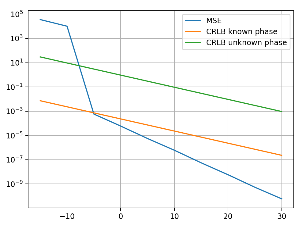
However, when I plot the Cramér-Rao Bound (CRB; orange curve below) $$ \mathrm{CRLB}\left( f \right) = \frac{3 \sigma^2}{\pi^2 N (N-1) (2N - 1)} \cdot f_\mathrm S^2 $$ (in [RiBo] equation (16), first case where phase is known and $n_0=0$ and $b_0=0$), the CRB stays above the mean squared error (MSE) of the ML estimator for larger SNRs. I also tried MUSIC (using spatial smoothing), which works slightly worse, but the CRB was still above.

Strangely, if I take the root of the MSE (RMSE), the CRB is below the CRB. But the variance shall be the MSE for unbiased estimators, not the RMSE. Probably I am doing something wrong here. Do you have any idea? The source code is here.

Maxmimum likelihood estimate and CRB

[RiBo] D. Rife and R. Boorstyn, "Single tone parameter estimation from discrete-time observations," in IEEE Transactions on Information Theory, vol. 20, no. 5, pp. 591-598, September 1974, doi: 10.1109/TIT.1974.1055282.

Solution:

I made a mistake in scaling the noise. It has to be scaled by $\sigma / \sqrt{2}$. That explains why the CRB and the estimator have different slopes on a log scale in the plot shown above.

$\endgroup$
2
  • $\begingroup$ What equation are you using for the CRLB formula from the paper? I'm not seeing that specific equation, I only see an $N(N^{2}-1)$ in the denominator. Also, notice equation 29. The maximizer of the likelihood function is not the real part of the DFT, but the unmodified periodogram. Furthermore, if you assume the periodogram is asymptotically Gaussian distributed, there is a straightforward calculation to compute the ML estimate of the true PSD from the periodogram. However, this shouldn't affect frequency estimation. $\endgroup$
    – Baddioes
    Commented Oct 4 at 5:17
  • 1
    $\begingroup$ If I understand the publication [RiBo] correctly, there are different estimators and CRBs for different scenarios. I was going for the case that the amplitude of the complex exponential is known ($b_0=1$ in the paper), the phase is known ($\theta=0$ in the paper), and the index of the first sample is zero ($n_0 = 0$ in the paper). So i used the ML estimator, mentioned in section III, C, 1) and the CRLB mentioned in the upper case of eq. (16). $\endgroup$
    – Balasana
    Commented Oct 4 at 10:11

2 Answers 2

3
$\begingroup$

You may have a look at Estimate Sine Frequency under White Noise.

The CRLB for a real harmonic signal is:

$$ \operatorname{var} \left( \hat{f} \right) \geq \frac{12}{ {\left( 2 \pi \right)}^{2} \cdot SNR \cdot \left( {N}^{3} - N \right) } {f}_{s}^{2} $$

For your case, a complex harmonic signal it is given by:

$$ \operatorname{var} \left( \hat{f} \right) \geq \frac{6}{ {\left( 2 \pi \right)}^{2} \cdot SNR \cdot \left( {N}^{3} - N \right) } {f}_{s}^{2} $$

In both the SNR is defined as:

$$ SNR = \frac{ {A}^{2} }{ {\sigma}_{n}^{2} } $$

Where $A$ is the amplitude of the harmonic signal and ${\sigma}_{n}^{2}$ is the AWGN noise variance.

You may have a look at the code to create such analysis in my StackExchange GitHub Repository (Look at the SignalProcessing\Q76644 folder). You may look at Q76644.m for the real harmonic case and Q76644C.m for the complex case.

$\endgroup$
8
  • $\begingroup$ According to the publication mentioned above, this is the CRB for the case that the phase in unknown. However, in my case the phase is known (i.e., zero). I also tried the derivation on my own and also came more or less to the same CRB (a different constant factor of: 3 instead of 6; see the Q variable in the paper.). $\endgroup$
    – Balasana
    Commented Oct 4 at 10:18
  • $\begingroup$ I don't think in real world you expect to know the phase :-). $\endgroup$
    – Royi
    Commented Oct 4 at 10:24
  • $\begingroup$ Yes, of course. This was just a toy example. However, the CRB for known and for unknown phase have the same slope on a log scale. They would just be shifted up or down. So that would not explain, why the MSE curve of the ML estimator (and as I tried also of the MUSIC estimator) has, on a log scale, a steeper negative slope than the CRB. Or at least, I do not see it. $\endgroup$
    – Balasana
    Commented Oct 4 at 10:32
  • $\begingroup$ @Balasana, Have you looked at the code from the link I posted? For me they collide perfectly with the CRLB I wrote. $\endgroup$
    – Royi
    Commented Oct 4 at 10:38
  • 1
    $\begingroup$ Thank you for the source code. When looking at it, I more or less immediately found my dumb mistake: I scaled the noise by $\sigma^2 / 2$ instead of $\sigma / \sqrt{2}$. $\endgroup$
    – Balasana
    Commented Oct 5 at 10:21
2
$\begingroup$

As I mentioned in my comment and as Royi pointed out, you should check your formula on the CRLB. Additionally, since you are using additive white Gaussian noise, the method of maximum likelihood (ML) converges to the non-linear least squares (NLS) solution. Furthermore, since you appear to be estimating a single frequency, I will also show that the NLS solution for a single frequency is the peak of the periodogram.

So, firstly defining the NLS problem. The NLS problem is defined as \begin{equation} f(\omega,\alpha,\phi) = \sum_{n=0}^{N-1}\left\lvert y[n]-\sum_{m=0}^{M-1}\alpha_{m}e^{j\left(\omega_{m}n+\phi_{m}\right)}\right\rvert^{2} \end{equation} We assume our signal is of the form \begin{equation} y = \psi(\gamma) + e \end{equation} where $e$ is white Gaussian noise, $\gamma$ is some unknown parameter, and $\psi(\gamma)$ is a deterministic function of $\gamma$. The pdf is then \begin{equation} p\left(y\,|\,\psi(\gamma),\sigma^{2}\right) = \frac{1}{(2\pi)^{N}\left(\sigma^{2}\right)^{N}}e^{-\frac{\left\lvert y-\psi(\gamma)\right\rvert^{2}}{2\sigma^{2}}} \end{equation} Taking the log we get \begin{align} \log\left(p\left(y\,|\,\psi(\gamma),\sigma^{2}\right)\right) &= -N\log(2\pi) - N\log(\sigma^{2})-\frac{\left\lvert y-\psi(\gamma)\right\rvert^{2}}{2\sigma^{2}} \\ -\log\left(p\left(y\,|\,\psi(\gamma),\sigma^{2}\right)\right) &= N\log(2\pi) + N\log(\sigma^{2})+\frac{\left\lvert y-\psi(\gamma)\right\rvert^{2}}{2\sigma^{2}} \end{align} We can choose to minimize the negative log-likelihood to maximize the log-likelihood. Taking the derivative with respect to $\sigma^{2}$ gives \begin{equation} \frac{\partial}{\partial\sigma^{2}}\left[-\log\left(p\left(y\,|\,\psi(\gamma),\sigma^{2}\right)\right)\right] = \frac{N}{\sigma^{2}} - \frac{\left\lvert y-\psi(\gamma)\right\rvert^{2}}{2\sigma^{4}} = 0 \end{equation} This gives \begin{equation} \hat{\sigma}^{2} = \frac{\left\lvert y-\psi(\gamma)\right\rvert^{2}}{N} \end{equation} Plugging this back in and gives \begin{equation} -\log\left(p\left(y\,|\,\psi(\gamma),\sigma^{2}\right)\right) = N\log(2\pi) + N\log\left(\frac{\left\lvert y-\psi(\gamma)\right\rvert^{2}}{N}\right)+N \end{equation} Since we wish to minimize the negative log-likelihood, and $\log()$ is a monotonically increasing function, we find that \begin{equation} \hat{\gamma} = \text{arg }\min_{\gamma}\left\lvert y-\psi(\gamma)\right\rvert^{2} \end{equation} which is precisely the NLS problem!

Now, let's reformulate the NLS problem into vector form. Let the following be true \begin{align} \beta_{m} &= \alpha_{m}e^{j\phi_{m}} \\ \beta &= \begin{bmatrix}\beta_{0} & \cdots & \beta_{M-1} \end{bmatrix} \\ \underline{y} &= \begin{bmatrix} y[0] & \cdots & y[N-1] \end{bmatrix} \\ \mathbf{B} &= \begin{bmatrix}1 & \cdots & 1 \\ \vdots & & \vdots \\ e^{j\omega_{0}(N-1)} & \cdots & e^{j\omega_{M-1}(N-1)} \end{bmatrix} \end{align} where $\mathbf{B}$ is a Vandermonde matrix. It can be shown 1 under certain assumptions that the NLS estimates of the frequencies are \begin{equation} \hat{\omega} = \text{arg }\max_{\omega}\left[\underline{y}^{H}\mathbf{B}\left(\mathbf{B}^{H}\mathbf{B}\right)^{-1}\mathbf{B}^{H}\underline{y}\right] \end{equation} In the case that there's only one true frequency, the matrix $\mathbf{B}$ becomes a steering vector to that frequency \begin{equation} \underline{a}(\omega) = \begin{bmatrix} 1 & e^{j\omega} & \cdots & e^{j\omega(N-1)} \end{bmatrix}^{T} \end{equation} The equation for $\hat{\omega}$ then becomes \begin{align} \hat{\omega} &= \text{arg }\max_{\omega} = \frac{\underline{y}^{H}\underline{a}(\omega)\underline{a}^{H}(\omega)\underline{y}}{\underline{a}^{H}(\omega)\underline{a}(\omega)} \\ &= \text{arg }\max_{\omega}\frac{\left\lvert\underline{a}^{H}(\omega)\underline{y}\right\rvert^{2}}{N} \end{align} which is the periodogram at frequency $\omega$ (see Computing modern spectral estimation techniques with FFTs for more details on why this is the case)!

There is a very in depth analysis in 1 on the bias and variance of the periodogram. Since the periodogram is asymptotically unbiased, the MSE will be the variance, which will be quite large (see more on that in Why is the sample spectrum considered inconsistent?). If you are interested in multiple frequencies, there is further analysis in 1 to show that the periodogram gives $\mathcal{O}\left(\frac{1}{N}\right)$ estimates of the NLS frequency estimates provided the finite sample periodogram has sufficient resolution such that all frequencies are spaced at least one DFT bin apart.

All of this is to show that you should absolutely expect the maximum likelihood estimate of the true frequencies, given a sinusoid in additive noise model, to be above the CRLB.

1 Stoica, P., & Moses, R. L. (2005). Spectral analysis of signals (Vol. 452, pp. 25-26). Upper Saddle River, NJ: Pearson Prentice Hall.

$\endgroup$
9
  • $\begingroup$ You wrote such a nice answer (+1). It is much better use the links title than just here or there. In few years the links might change, yet the text is always searchable. $\endgroup$
    – Royi
    Commented Oct 4 at 8:03
  • $\begingroup$ @Royi thanks! I will update the links. $\endgroup$
    – Baddioes
    Commented Oct 4 at 8:05
  • 1
    $\begingroup$ I already did that for you. $\endgroup$
    – Royi
    Commented Oct 4 at 8:06
  • $\begingroup$ @Royi thanks. The answer hadn't yet updated on my end, so sorry for the confusion. $\endgroup$
    – Baddioes
    Commented Oct 4 at 8:08
  • $\begingroup$ Cool, thanks! Will try out! :-) (Does not answer the question, why the CRB descends less rapid than the MSE in my implementation, but it's nice.) $\endgroup$
    – Balasana
    Commented Oct 4 at 10:35

Your Answer

By clicking “Post Your Answer”, you agree to our terms of service and acknowledge you have read our privacy policy.

Not the answer you're looking for? Browse other questions tagged or ask your own question.