Real Data Complex Transfer Function using H0, H1, H2 Estimators

Question

BACKGROUND:

This question is attempting to consolidate material discussed in two previous topics. These are:

Understanding the H1 and H2 estimators @Pontus S

Frequency-domain deconvolution: "Direct" filtering vs "Wiener" filtering

I am estimating Complex Frequency-Domain Transfer Functions.

I will call the frequency-domain system X H = Y.

I am comparing estimators:

H0 = Y/X (i.e. direct frequency domain division OUTPUT/INPUT)

H1 = (YX*) / (XX*) (* is conjugate, H1 is supposedly best for output noise)

H2 = (YY*) / (XY*) (best for input noise)

Note that I only have a single recording of each experiment, so I cannot do any averaging of the spectra in H1, and H2.

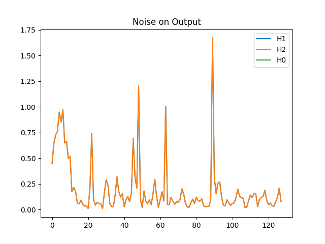
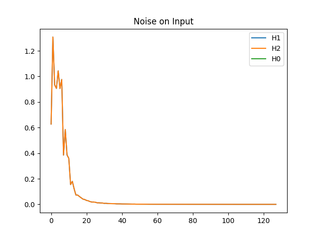
For synthetic and real data, the three estimates appear identical. (Not surprising as they are mathematically identical, as pointed out by @Pontus in Q 71811.)

QUESTIONS:

1. Is the reason my H0, H1, H2 estimates are the same because I am not able to do any averaging in the spectra. Hence I am not reducing the influence of noise.
2. In this situation is there anything to be gained by using H1, H2. rather than just H0 (Direct division)?

================================

Feedback to @V.V.T.

Thanks very much for the effort you have put into this. It is appreciated. However, your code is investigating a different problem to the one in my post. You are feeding three different signals to the three estimators. My question relates to real data, where the noise is already added. If you modify your code slightly you will see what I mean. Here is what you get when you apply the three estimators all to same signal, with noise on the output. The three estimates plot on top of each other. i.e. they are identical

Similarly if the three estimators are applied to the signal with noise on the input, the estimates plot over the top of each other.

CODE:
import numpy as np
import scipy
from scipy import signal
import matplotlib.pyplot as plt
from scipy.signal import max_len_seq
#from scipy.fft import fft, ifft

# 'INPUT' sequence
x = max_len_seq(8)[0]*2.0-1.0
plt.figure(0)
plt.plot(x)
plt.show()

lx=len(x)

# Comb filter
b, a = signal.butter(3, 0.05)

#awgn noise
z = np.random.normal(0, 0.1, len(x))

y = signal.lfilter(b, a, x)
# signal with noise on  output############
yn = y + z
plt.plot(yn)
plt.show()
#H1 estimator auto/cross spectral densities pxx pxy
_, pxy = signal.csd(x,yn)
_, pxx = signal.csd(x,x)
H1 = np.divide(pxy,pxx)
plt.figure(1)
plt.title("Noise on Output")
plt.plot(abs(H1), label="H1")
#H2 Estimator
f, pyy = signal.csd(yn,yn)
f1, pyx = signal.csd(yn,x)
H2 = np.divide(pyy,pyx)
plt.plot(abs(H2), label="H2")

#H0 estimator (Spectral division)
flat=np.ones(lx,float)  #just to enable consistent use of csd
                        #to get the spectrum of x, and yn
_, px = signal.csd(x,flat)
_, pyn= signal.csd(yn,flat)
H0 = np.divide(pyn,px)
plt.plot(abs(H0), label="H0")

plt.legend()
plt.show()

     
#  signal with  noise on input####################3
xn = x + z
y2 = signal.lfilter(b, a, xn)
_, pxy = signal.csd(xn,y2)
_, pxx = signal.csd(xn,xn)

#H1 Estimator

H1 = np.divide(pxy,pxx)
plt.figure(2)
plt.title("Noise on Input")
plt.plot(abs(H1), label="H1")

#H2 estimator, auto/cross spectral densities pyy pyx

f, pyy = signal.csd(y2,y2)
f1, pyx = signal.csd(y2,xn)
H2 = np.divide(pyy,pyx)
plt.plot(abs(H2), label="H2")

_, px = signal.csd(xn,flat)
_, pyn= signal.csd(y2,flat)
H0 = np.divide(pyn,px)
plt.plot(abs(H0), label="H0")


plt.legend()

plt.show()

exit()

I am not very familiar with the signal.csd routine, but it is possible that with the short sequence used here (255) there is no averaging/windowing being done. This is my situation (no spectral averaging). Note that when the signal is made longer, using the csd code some differences emerge, and this may be because spectral averaging is being done in csd. This is what what suggested by @Pontus in his final comment (#74836), and the purpose of my question was to see if he or anyone else could confirm this with real-data experience.

Again thanks very much for your time and effort. I have upticked your answer to reflect your input.

Answer 1

UPDATE

Python's signal.csd routine, as it is used in my code, don't work miracles, at least in the sense you would expect ("but it is possible that with the short sequence used here (255) there is no averaging/windowing being done" -- as if it does averaging/windowing for >255 sequences). From the code you can see that, when presented only the input and output data, the program has no means to separate the output into pure signal plus noise and can only do its best to recover the transfer function of the LTI system from its input and output data as if the output signal plus noise is a newly defined output signal and there is no noise in the system at all -- to solve the ill-posed problem of deconvolution.

We can re-formulate the problem: multiple realizations of the LTI system's output with noise at the output are given for an identical input data. Providing that there is no noise at input, what is the best estimate for the system transfer function? The code below solves the problem with 64 realizations given.

import numpy as np
from scipy import signal
import matplotlib.pyplot as plt
from scipy.signal import max_len_seq
from scipy.fft import fft, ifft

# 'INPUT' sequence
x = max_len_seq(8)[0]*2.0-1.0
_, pxx = signal.csd(x,x)

# linear filter
b, a = signal.butter(3, 0.05)

# noiseless output
y = signal.lfilter(b, a, x)

z = np.random.normal(0, 0.1, len(x))
# add noise to output
yn = y + z
_, pxy = signal.csd(x,yn)
H1 = np.divide(pxy,pxx)
plt.figure(1)
plt.title("H1: a noise realization added to output")
plt.plot(H1)

# average output noise over ensemble
yn = y + z/64
for iter in range(1,64):
  yn = yn + np.random.normal(0, 0.1, len(x))/64

# cross psd with averaged output over ensemble
_, pxy = signal.csd(x,yn)

#H1 estimator 
H1 = np.divide(pxy,pxx)
plt.figure(2)
plt.title("H1: yn averaged over sixty four realizations of noise at output")
plt.plot(H1)

#spectral division
X = fft(x)
Y = fft(y)
H0 = np.divide(Y, X)
plt.figure(3)
plt.plot(H0[0:len(H0)//2])

#draw plots
plt.show()

And it is exactly what ZR Han posited in the answer to your question.

But pay attention to the conditional "as it is used in my code": you can employ the independence of noise component samples to avail and, to some degree, replace averaging over a signal ensemble by averaging over these i.i.d. variables of a unique signal realization. This is the ergodic theory in action: under certain conditions, averaging over ensemble is equivalent to averaging over time.

The scipy.signal.csd function has the optional 'window' parameter. By default this parameter is 'hann', the window length of 256, but I doubt that default parameters result in the noise handling in the way required for estimators, that is, averaging over independent realizations. However, there is a window value, 'dpss', which can be used to apply said 'ergodicity' to your avail. I would not bore you with a lecture on this approach in my rendering, you can read elsewhere about the technique called a "multitaper" method.

To my knowledge, there is no readily available scipy's implementation of multitaper. However, you can implement it for yourself.

Start with a simpler task of implementing the psd calculation with multitaper. For the toy problem you can take an unsolved task from the question How to accurately compute the Winger-Ville Distribution of an exponential. The OP was upset that he cannot replicate numerically the Wigner-Ville distribution. The principal reason was incorrect generation of the Wiener process realization, but in the end he required the precise coincidence including the distribution tails, and it is impossible with spectral division exactly for the same reason that you receive "the same result" for estimators: the averaging over ensemble is required. You can use the distribution tail suppression task to acquire skill in multitaper application. You can start with a multitaper implementation for PSD calculation -- for example, taken from github, as e.g. https://github.com/xaratustrah/multitaper or else -- and later to extend it or write your own implementation for cross channel spectral distribution calculation. Or maybe you would accommodate scipy's csd, using window='dpss', into your solution from the beginning. If you engage in this task, make known to dsp.SE users when you post your solution to github.