2
$\begingroup$

Pg. 223 claims so, yet my results via DFT differ:

Is the textbook wrong?


My attempted explanations: (code)

  1. DFT vs DTFT: "frequency response" is computed via latter. Still, DFT should resemble a sampled DTFT.

  2. DFT time-domain periodicity, whereas DTFT assumes aperiodic, or "repeats at infinity" with infinite zero-padding.

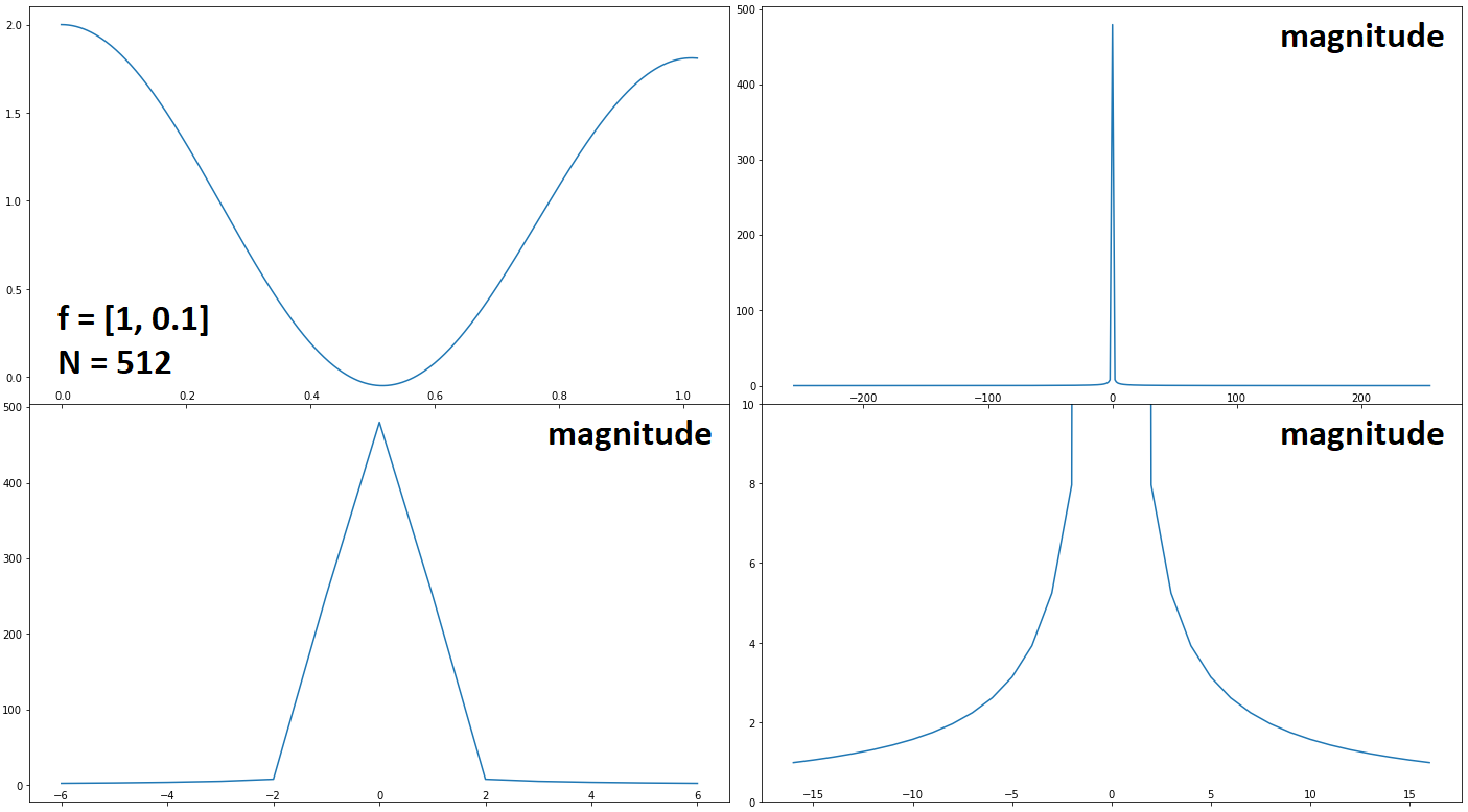
To address each, I try greater N, and zero-padding - below. Zero-padding appears to correct phase (quadratic if unrolled), and more samples tend to flatten the magnitude for an ever-growing portion of frequencies to the right.

I figure, in the limit N -> inf, the amplitude spike has zero width (like in Gibbs) - but this appears contradicted in the "large N long padding" case, where a nontrivial portion of the amplitude decays with oscillations. Further, the left peak appears to scale with N, behaving more like an impulse in the limit, which won't yield zero energy as in Gibbs phenomenon.


Update: turns out magnitude doesn't spike, but rather decays exponentially, which is far from the expected horizontal line - and, the phase is linear:


Note: see comments below accepted answer for further info.

$\endgroup$

3 Answers 3

3
$\begingroup$

The book is not wrong, but it does present the concepts on LFM in a clunky manner and can be misleading. The book presents the analytical expression for the LFM spectrum, which is an approximation. It also plays with the plot views and most likely unwraps the phase angles, which is usually required to see the phases you expect.

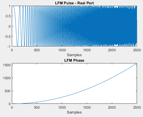
Usually when you're introducing LFM, you'll show the modulated pulse itself as well as the phase progression in the time-domain. The analytical expressions in the time domain is all you need to observe the linear frequency and therefore quadratic phase nature of LFM. Doing this in the frequency-domain just tends to introduce more confusion. An example of the time-domain LFM pulse and its phase is shown below.

enter image description here

When deriving the expression for the Fourier transform of an LFM pulse, you do indeed yield a magnitude of 1 over the bandwidth of the pulse. This is intuitively satisfying because you have the same contribution from each frequency over the bandwidth.

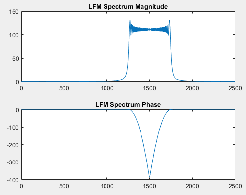
Confusion does occur however when one goes to plot this if they expect a constant frequency response. With any practical LFM spectrum plot, even with very long pulse widths, one should expect a ripple effect which you have already identified. The quadratic nature of the phase is still captured in the DFT. The spectrum of the LFM pulse from above is shown below.

enter image description here

I haven't tried your code, but it might be that you just need to zoom in the proper areas and unwrap the phases to see what you want. Provided is the MATLAB code to produce the plots to help you in converting it to python.

%% LFM - Time and Frequency Domain

% Sampling
Fs = 50e6;

% Pulse parameters
tau = 50e-6;
bandWidth = 10e6;
alpha = bandWidth/tau;

% Define waveform
t = 0:1/Fs:tau - 1/Fs;
fmcwPulse = exp(1i*pi*alpha.*t.^2); % Complex transmitted LFM waveform

% Plot
figure;
subplot(2, 1, 1);
plot(real(fmcwPulse));
xlabel("Samples");
title("LFM Pulse - Real Part");

subplot(2, 1, 2);
plot(unwrap(angle(fmcwPulse)));
xlabel("Samples");
title("LFM Phase");

figure;
subplot(2, 1, 1);
plot(abs(fftshift(fft(fmcwPulse))));
title("LFM Spectrum Magnitude");

subplot(2, 1, 2);
plot(unwrap(angle(fftshift(fft(fmcwPulse)))));
title("LFM Spectrum Phase");

Update

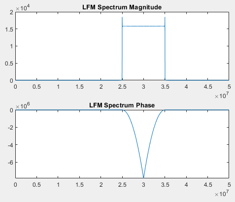
Modifying the code above so that $\tau = 1 \space s$, which is relatively long, yields a spectrum closer to the ideal flat spectrum that one would expect analytically. The spectrum is shown below.

enter image description here

$\endgroup$
13
  • $\begingroup$ "even with very long pulse widths, one should expect a ripple effect" - why? What prevents the magnitude from converging to a straight line as N -> inf? As I further noted, the energy of the magnitude spike doesn't near zero with increasing N, which it must if we are to conclude "it's because N is finite". It isn't even a spike, but worse, and unwrapped phase turned out linear - question updated. $\endgroup$ Commented Sep 3, 2020 at 0:00
  • $\begingroup$ @OverLordGoldDragon Technically yes, if you increase the pulse width you will approach a flat spectrum but is not practical. Take a look at the code I posted. There might be something wrong with how you have implemented it in Python. $\endgroup$
    – Envidia
    Commented Sep 3, 2020 at 0:04
  • $\begingroup$ You presented a misleading (if not false) example with the topmost chirp; the phase shown is that of the imaginary component relative to real component of a 'complex chirp' (which isn't even the phase of the chirp itself); "the phase" refers to that of the sinusoidal frequency components, doesn't it? So it must first be transformed, and be real to begin with. Further, my code is fine; it uses numpy's fft to find real DFT, then finds magnitude as sqrt(imag^2 + real^2). Are you able to flatten the magnitude in MATLAB? $\endgroup$ Commented Sep 3, 2020 at 0:32
  • $\begingroup$ @ I don't understand what you mean that "which isn't even the phase of the chirp itself". This is by definition the phase of the LFM pulse. Recall that the instantaneous frequency of a sinusoid is the derivative of the phase. This is why LFM chirps are called to be quadratic phase, which is where their linear frequency comes from. I'm going to update the post to include a long chirp that yields a flatter spectrum. $\endgroup$
    – Envidia
    Commented Sep 3, 2020 at 0:41
  • $\begingroup$ We aren't on the same page then, as the definition I follow is within the context of the textbook, which hasn't presented what you speak of. It's a chapter on DFT, so I can only understand "phase" as that of a signal's frequency components. I can't attribute much meaning to your usage of phase, however; looks like the phase of a signal whose DFT's real & imaginary components are chirp. Have a reading reference? $\endgroup$ Commented Sep 3, 2020 at 0:51
0
$\begingroup$

The short answer to "why do my DFT responses differ?" is that you have a chirp with a very small time-bandwidth product. Chirps that last longer in time, or sweep over a larger frequency range, become closer to an ideal chirp.
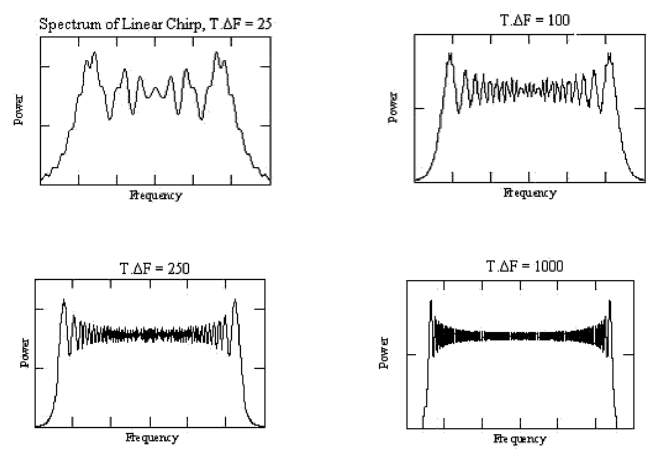
enter image description here

(from https://en.wikipedia.org/wiki/Chirp_spectrum, though the page is also somewhat confusing overall)

The shape of the rect. function in frequency has nothing to do with the sampling frequency $f_s$ (assuming you're sampling sufficiently faster than the Nyquist frequency), and nothing to do with adding extra zero padding.

I agree that the original book was confusing by drawing the graph as a straight line instead of a rectangle. The post by @Envidia already illustrates how a larger time-bandwidth product will make the frequency response approach the ideal rect function, with the Gibb's ringing being unavoidable for non-infinite discrete signals.

Re: the puzzle "why does the frequency 10 sinusoid move slower than the frequency 1->2 chirp?"

I just wanted to include this because I've made the same mistake and seen new signal processing students do this too. Most signal processing texts have mostly math formulas with continuous variables, so it's easy to think writing cos(2 * pi * f * t) in Python or MATLAB would mean that your angular phase is $2 \pi f t$ and therefore frequency is the variable f, regardless of what the code variables t and f hold.

Though it seems like doing f = linspace(1, 2); cos(2 * pi * f * t) means that the cosine is "sweeping frequency from 1 to 2", the instantaneous frequency of $\cos(\phi(t))$ is the derivative of $\phi$, $\dot{\phi}(t)$ (as noted above).

Therefore, doing this only works if you start time at 0, and have f = linspace(1, 2). This will get the plot you expect for the phase (the argument to the cosine) and the cosine itself:
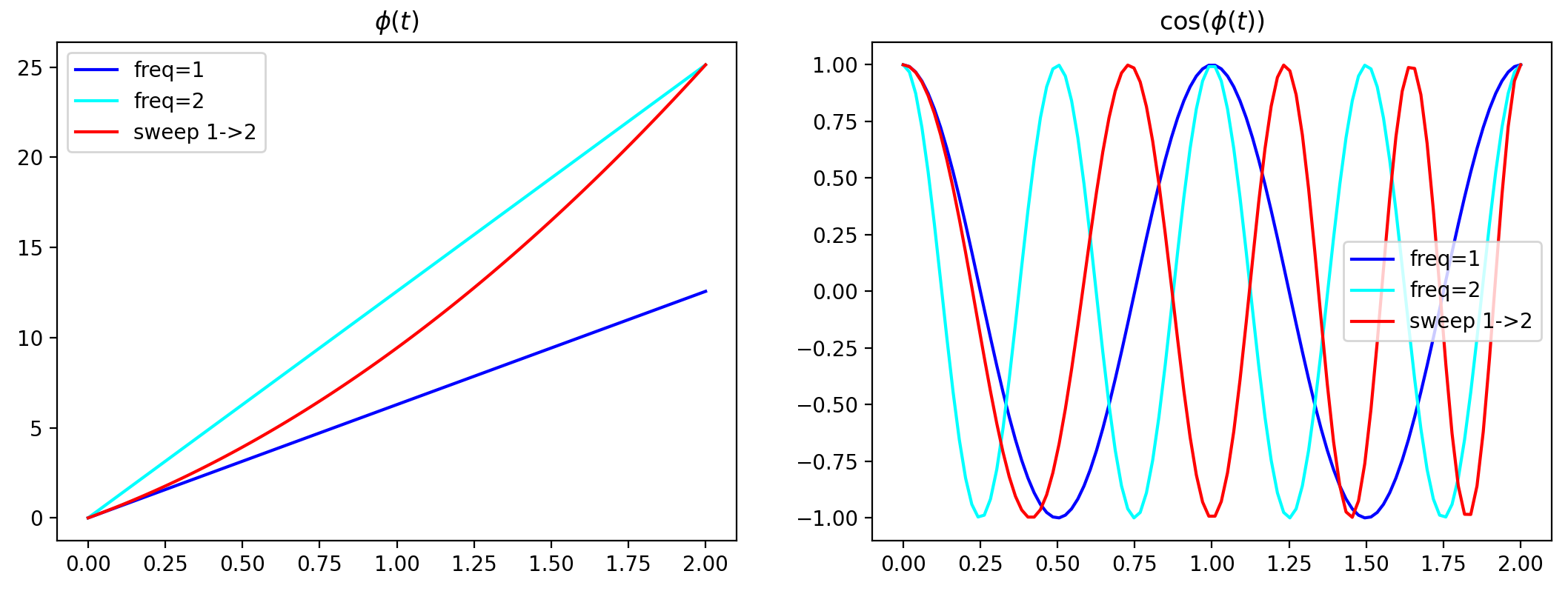
enter image description here

BUT if you have something like t = linspace(1, 2, n), the phase that sweeps the same frequency range is no longer just 2 * pi * f * t.

To sweep from $f_{1}(t)$ to $f_2(t)$, you'll want to create the function $f(t)$ as a line starting from $f_{1}(t)$ to $f_2(t)$. Then use the values of $t$ you're considering and solve for the slope and intercept. This ensures that the slope of the phase matches the frequencies you are trying to sweep over.

Here's an example of the difference, using slightly different numbers (If you are trying to "sweep frequency from 1 to 2", but the time your looking at starts at 1 instead of 0 and goes for 1 second). The left are phases, and right are cos(phase) plots to see how fast they wiggle. The wrong way in red is doing t = linspace(1, 2); f = linspace(1, 2); phase_wrong = 2 * pi * f * t. By comparing with the constant-slope-phase of 2, which definitely has a frequency of 2 everywhere, you can see that this method goes something with a steeper slope than 2, so it's not sweeping frequency from 1 to 2.
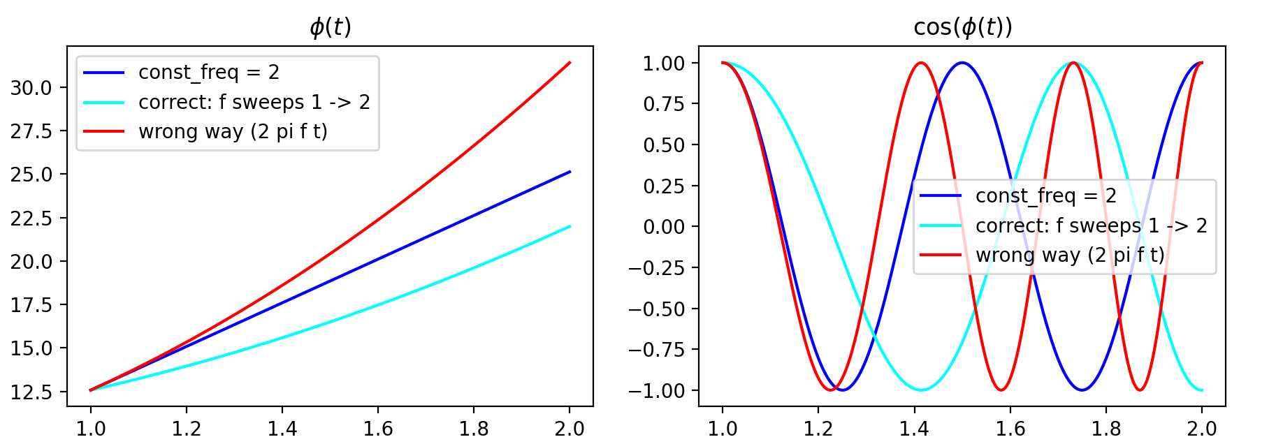
enter image description here

(code for the plot:)

import matplotlib.pyplot as plt
from numpy import pi, cos, linspace

n = 500
t = linspace(0, 2, n)
f = linspace(1, 2, n)

fig, axes = plt.subplots(1, 2)

ax = axes[0]
ax.plot(t, 2 * pi * 1 * t, c="b", label="freq=1")
ax.plot(t, 2 * pi * 2 * t, c="cyan", label="freq=2")
ax.plot(t, 2 * pi * f * t, c="red", label="sweep 1->2")

ax.set_title(r"$\phi(t)$")
ax.legend()

ax = axes[1]
ax.plot(t, cos(2 * pi * 1 * t), c="b", label="freq=1")
ax.plot(t, cos(2 * pi * 2 * t), c="cyan", label="freq=2")
ax.plot(t, cos(2 * pi * f * t), c="red", label="sweep 1->2")

ax.set_title(r"$\cos(\phi(t))$")
ax.legend()


fig, axes = plt.subplots(1, 2)
t = linspace(1, 2, n)
phi_right = pi * (t ** 2 - 1)

f = linspace(1, 2, n)
phi_wrong = 2 * pi * f * t

# Compare to a constant freq (straight phase line)
const_freq = 2

ax = axes[0]
ax.plot(t, 2 * pi * const_freq * t, c="b", label=f"{const_freq = }")
# Make it start at same spot as constant freq phase line
offset1 = phi_right[0] - 2 * pi * const_freq * t[0]
ax.plot(t, phi_right - offset1, c="cyan", label="correct: f sweeps 1 -> 2")
offset2 = phi_wrong[0] - 2 * pi * const_freq * t[0]
ax.plot(t, phi_wrong - offset2, c="red", label="wrong way (2 pi f t)")
ax.set_title(r"$\phi(t)$")
ax.legend()

ax = axes[1]
ax.plot(t, cos(2 * pi * const_freq * t), c="b", label=f"{const_freq = }")
ax.plot(t, cos(phi_right), c="cyan", label="correct: f sweeps 1 -> 2")
ax.plot(t, cos(phi_wrong), c="red", label="wrong way (2 pi f t)")
ax.legend()
ax.set_title(r"$\cos(\phi(t))$")

(@OverLordGoldDragon also pointed out more real code examples of his, which can be more useful than the math-only formulas: https://overlordgolddragon.github.io/test-signals/#signal-general-forms-derivations )

$\endgroup$
1
  • $\begingroup$ I was able to produce a "perfect" chirp spectrum here, but never looked into what made it perfect. The DFT can be tricky; helps to know what exactly its coefficients mean. My guess is some convenient discrete-continuous lineup occurs; may look into some day. $\endgroup$ Commented Feb 26, 2021 at 21:47
-1
$\begingroup$

The textbook is wrong, or very misleading depending on interpretation. The frequency response is square - or, constant over the swept frequency. Assuming an ideal chirp system which can scale up $f$ to any arbitrary duration $t$ (infinite bandwidth);, then the magnitude is a square of infinite width - which happens to be the same as plain "constant".

What follows are a number of related descriptions; thanks to Envidia for helpful discussion - refer to his answer for complex chirp plots.


  • Phase (of chirp): quadratic. Must be careful with what's meant by "phase"; the instantaneous, i.e. the complete input, $\phi(t)$: $\cos(\phi(t))$. The instantaneous frequency of $\cos(t^2)$ isn't $t$, but $t/2$; see here.

  • Phase (of freq response): parabolic, with half-parabolas symmetric about and adjacent to the spike at $f_{\text{max}}/2$. So is the textbook wrong? For any physical, finite chirp system, yes - but book again assumes an ideal system with an infinite frequency swept, so the "peak" sits at infinity, rendering the phase a true parabola.

  • Magnitude (of chirp): for a complex chirp, it's unity / peak amplitude, as for any complex signal with shared inst. phase ($\sin^2 + \cos^2$). For a real chirp, it's the abs. value of amplitude.

  • Magnitude (of freq response): why the ripples? Because $f$ sweeps fractional frequencies, which are represented as combinations of nearby and higher frequencies when a given frequency doesn't last long enough (for a chirp, each lasts for a mere one sample).

    • Symmetry: real -> even about DC; complex -> asymmetric, no negative frequencies.

I've used mainly this code for visualizing various scenarios. As a puzzle (to readers; I already understand) for understanding the topmost bullet point, I pose the following: how does a frequency swept from 1 to 2 complete more cycles than a signal with $f=10$ over the same period? What if instead $t$ is from 11.9 to 12.0?

Don't look at the Wiki, or especially this code, as both answer the question (for most part).

$\endgroup$
7
  • $\begingroup$ Take this result and then try plotting it over the interval [0, 1] but then zoom in to the interval [0.9, 1]. What do you notice? $\endgroup$
    – Envidia
    Commented Sep 8, 2020 at 16:46
  • $\begingroup$ @Envidia Edited to clarify I already understand it - unless you're suggesting it for other readers. $\endgroup$ Commented Sep 8, 2020 at 17:04
  • $\begingroup$ So you have a good handle on why setting the time vector from [0, 0.1] shows that the swept signal completes less cycles over the same period? $\endgroup$
    – Envidia
    Commented Sep 8, 2020 at 17:45
  • $\begingroup$ @Envidia Total handle; derived ("reinvented") this via a thought experiment of a physical handle powered electrically, where source jumps from $f=1$ to $=2$. The results are more absurd the larger $t$ is, and that it's dependent on $t$ at all is itself absurd. I used to not be a fan of discrete stuff - but finally relearning it properly, I'm liking it even more than continuous, as it's more "inspectable" and truer to reality in some regards. $\endgroup$ Commented Sep 8, 2020 at 17:56
  • 1
    $\begingroup$ @ScottStaniewicz The best way to understand the phenomenon is by understanding the DFT; I wouldn't write up this answer with my current knowledge. I've also coded the most general forms of linear, exponential, and hyperbolic chirps here, derived here. $\endgroup$ Commented Feb 26, 2021 at 20:29

Your Answer

By clicking “Post Your Answer”, you agree to our terms of service and acknowledge you have read our privacy policy.

Not the answer you're looking for? Browse other questions tagged or ask your own question.