1
$\begingroup$

Edit

As for window weighted mean, this is known as Birkhoff averaging. In the case of quasiperiodic signals, such averaging is superconvergent. Weighting by $\exp\left(\frac{1}{t^n (t - 1)^n}\right)$ with $n=1$ is particulary efficient.

Super convergence of ergodic averages for quasiperiodic orbits

End

Consider real signal of the form: $$ \begin{align*} x(n) = &\sum_{m=1}^{M} \left( c_m \cos(2\pi f_m n) + s_m \sin(2\pi f_m n) \right) =\\ &\sum_{m=1}^{M} a_m \cos(2\pi f_m n + \phi_m) \end{align*} $$ where signal values of $x(n)$ are known for $n = 1,\dots, N >> M$ and some frequencies $f_m$ are known real numbers in $(0.0,0.5)$.

What is the best way to estimate $c_m$ and $s_m$ real parameters?

Estimation of the form: $$c_m + j s_m = 2 \frac{\displaystyle\sum_{n=1}^{N} x(n) \exp(2 \pi j f_m n)}{N}$$ is not very accurate ($j^2=-1$), but windowing (e.g. cosine window) improves estimation accuracy significantly: $$c_m + j s_m = 2 \frac{\displaystyle\sum_{n=1}^{N} w(n) x(n) \exp(2 \pi j f_m n)}{\displaystyle\sum_{n=1}^{N} w(n)}$$

Why window is so effective here? Is it some kind of well-known formula?

The least-squares method also gives good results if frequencies are known for all terms.

Are there any other good methods for the case when not all frequencies are known? Perhaps based on SVD or some kind of orthogonalization.

Test code in Mathematica:

F1 = 0.123000 ;
F2 = 0.312874 ;

LENGTH = 1024 ;
RANGE = Range[LENGTH] ;

SIGNAL = 0.0 ;
SIGNAL = SIGNAL + 1.0*Cos[2*Pi*F1*RANGE] + 0.5*Sin[2*Pi*F1*RANGE] ;
SIGNAL = SIGNAL + 0.05*Cos[2*Pi*F2*RANGE] + 0.01*Sin[2*Pi*F2*RANGE] ;

WINDOW = HannWindow[N[Rescale[Range[LENGTH],{1,LENGTH},{-1,1}]]]^2 ;

(* NO WINDOW *)
2*(Total[SIGNAL*Exp[2*Pi*I*F1*RANGE]]/LENGTH)               
2*(Total[SIGNAL*Exp[2*Pi*I*F2*RANGE]]/LENGTH)               
(* OUTPUT: 0.9994929536863852`\[VeryThinSpace]+0.49994639046951617` I *)
(* OUTPUT: 0.04819835064062154`\[VeryThinSpace]+0.012127390241918076` I *)

(* WITH WINDOW *)
2*(Total[SIGNAL*WINDOW*Exp[2*Pi*I*F1*RANGE]]/Total[WINDOW]) 
2*(Total[SIGNAL*WINDOW*Exp[2*Pi*I*F2*RANGE]]/Total[WINDOW])
(* OUTPUT: 0.9999999999775656`\[VeryThinSpace]+0.5000000000025541` I *)
(* OUTPUT: 0.05000000004559643`\[VeryThinSpace]+0.009999999958900167` I *)

(* LEAST SQUARES *)
(* ONE KNOWN *)
LeastSquares[{Cos[2*Pi*F1*RANGE],Sin[2*Pi*F1*RANGE]}//Transpose,SIGNAL]
(* ALL KNOWN *)
LeastSquares[{Cos[2*Pi*F1*RANGE],Sin[2*Pi*F1*RANGE],Cos[2*Pi*F2*RANGE],Sin[2*Pi*F2*RANGE]}//Transpose,SIGNAL]
(* OUTPUT: {0.999957445314386`,0.4999499273288035`} *)
(* OUTPUT: {1.`,0.49999999999999983`,0.05000000000000022`,0.010000000000000056`} *)
$\endgroup$
17
  • $\begingroup$ @Royi, LS is good when all freqs are known, but expression with window is good in any case. I'm missing on 'canonical' procedure to determine parameters. Also, a reference on why window works here. $\endgroup$
    – I.M.
    Commented Sep 11, 2020 at 6:06
  • $\begingroup$ @Royi, not all frequencies are known in general. $\endgroup$
    – I.M.
    Commented Sep 11, 2020 at 6:25
  • $\begingroup$ My mistake, I missed that you wrote "some frequencies". $\endgroup$
    – Royi
    Commented Sep 11, 2020 at 6:53
  • 1
    $\begingroup$ This problem is known as "multiple tone decomposition". There are lots of approaches. The best (IMO) being what I am working up towards in my blog articles which will converge rapidly to an exact solution. dsprelated.com/blogs-1/nf/Cedron_Dawg.php The multiple tone decomposition involves iteratively estimating each tone and removing them from the mix except for one and re-estimating the sole remaining tone. Repeat for each tone. My equations allow this to be done efficiently in the spectrum instead of the time domain. $\endgroup$ Commented Sep 11, 2020 at 15:07
  • 1
    $\begingroup$ @CedronDawg, thank you for your help, I'll look through your posts. $\endgroup$
    – I.M.
    Commented Sep 11, 2020 at 16:12

2 Answers 2

3
$\begingroup$

Bottom Line: The OP is experiencing the effects of spectral leakage and the primary motivation for windowing with the Discrete Fourier Transform. The reason the windowing approach achieves much better estimation accuracy is explained as follows:

The OP's equation is a sum of real sinusoids, and his estimator to determine those sinusoids is a form of the Discrete Fourier Transform (DFT). Without additional windowing (which is a rectangular window) it is well understood that the DFT suffers from a considerable amount of spectral leakage, in that the Kernel of the rectangular window (the Discrete-Time Fourier Transform or DTFT of the rectangular window which is of the form of an aliased Sinc function) convolves in frequency with the underlying two impulses in frequency of each real sinusoid. Since the aliased Sinc function decreases relatively gradually with frequency offset from the location of the impulses representing the tones, and has such high side-lobes, many other frequency bins are affected causing errors in their own measurements (and a significant decrease in dynamic range or the ability to detect a lower level tone in the presence of a strong one). Windows are selected that have the property of much lower side-lobe levels, and roll-off much faster in frequency, which therefore causes any given tone to have much less impact on the estimation of other tones present.

This is made much clearer if we observe the DTFT instead of the DFT, as the DTFT is a continuous function of frequency and the DFT is samples on this continuous function. By observing the DTFT we can more easily get the full intuitive picture of what is being described above. Further we also see how approximating the DTFT (through zero-padding prior to doing the DFT) can also be used to approximate the frequencies). I show this with plots of the OP's original frequencies where we can see the effect of the windowing directly:

First consider the OP's example of 1024 samples with just F1 alone with and without additional windowing. First without additional windowing (rectangular window) The log magnitude plot of the DTFT with the corresponding 1024 DFT samples of just F1 is given in the plot below:

This is specifically the DTFT of

$$sig1 = 1.0\cos(2\pi f_1 n) + 0.5\sin(2\pi f_1 n)$$

for n = 0 to 1023. And f1 = 0.123

(Note: the above is just a single tone at $f1$ with additional phase shift as can be derived from the relationship $a\cos(x)+b\cos(x) = \sqrt{a^2+b^2}\cos(x-\tan^{-1}(b/a))$

Magnitude Spectrum of F1 Signal Only - Rectangular Window DTFT of F1
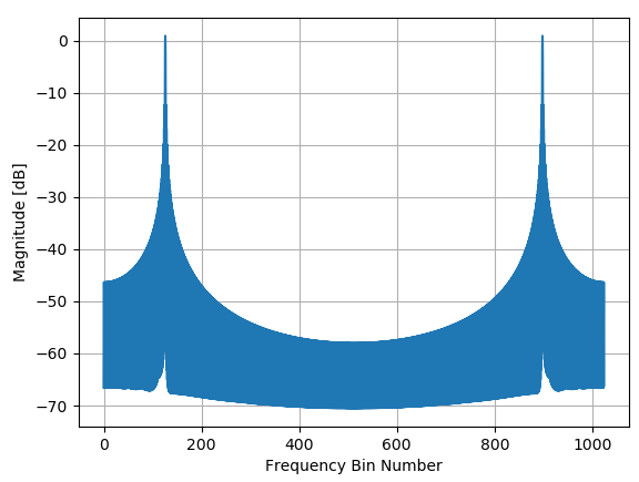
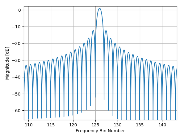
If we zoom in on one of the spectral peaks, we can clearly see the Sinc shaped Kernel (in this case given the number of samples the aliasing would be very small so this is a very close approximation of an actual Sinc) that has convolved with the underlying impulse that would be at the F1 frequency location, and we see the spectral leakage and how it affects the other frequency locations. F1 as 0.123 is very close to bin number 126 as given by $1024 \times .123 = 125.952$.

Zoom In on F1 Peak Location Zoom in of DTFT
Below I show the two frequency components as the OP has used, but still as separate signals to demonstrate how the spectral leakage of each will effect the measurement of the other.

This is specifically

$$sig1 = 1.0\cos(2\pi f_1 n) + 0.5\sin(2\pi f_1 n)$$ $$sig2 = 0.05\cos(2\pi f_2 n) + 0.01\sin(2\pi f_2 n)$$

For n = 0 to 1023 and f1 = 0.123 and f2 = 0.312874

Magnitude Spectrum of F1 and F2 Signals (Separate) - Rectangular Window DTFT of both F1 and F2 separately
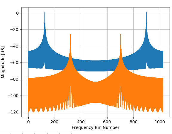
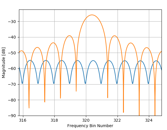
Notice if we zoom in on the peak for F2 how significant the leakage from F1 is will effect the estimate of the magnitude for F2, given that the leakage from F1 is only 29 dB lower! If the magnitude of F2 was made lower, the resulting error would be even more pronounced. (Also notice how with the DTFT we can locate the F2 frequency precisely at its fractional bin location of $1024 \times 0.312874 \approx 320.3830$ which is where the peak of the orange curve in the plot below would be located, but once combined with the F2 signal given by the blue curve, this would cause a frequency error as well since the peak of the blue curve happens slightly to the right of the orange F1 curve.

Zoom In on F2 Peak Location - With Rectangular Window Zoom in of DTFT of both F1 and F2 separately
If we then compute the DTFT of the composite waveform with both F1 and F2, we see the resulting amplitude and frequency error in vicinity of the F2 Peak location as shown in the plot below (where Green is the DTFT of the composite waveform summing both F1 and F2 components).
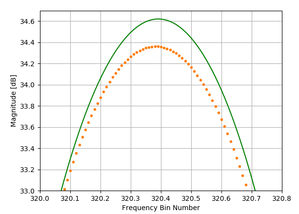
Zoom in on F2 Peak of composite - With Rectangular Window

This error is predicted by the coherent sum of the two waveforms and thus can be predicted from rectangular window Kernel and knowledge of the relative amplitude and frequency offsets of the two signals. Given the waveforms are complex the phase of the components will impact the summation result (thus the inteference could feasibly reduce or increase the amplitude of the affected component).

In this example the following were the signal contributions at the F2 peak location (not in dB scale as above to show the summation directly).

F2 alone at bin 320.38: magnitude = 52.10 (given as 52.00 -j3.26)

F1 alone at bin 320.38: magnitude = 1.70 (given as 1.42-j0.94)

F1 + F2 at bin 320.38: magnitude = 53.58 (given as 53.42-j4.19)

Where F1 + F2 as measured is predicted by the sum of F1 and F2 alone when the complex components are added.

Finally if we observe the above plot with the use of windowing (we'll use the same Hann window the OP used) we can see the significant reduction in spectral leakage and then exactly how this would contributed to a better estimation of both the frequency and magnitude of the underlying signals.

Magnitude Spectrum of F1 and F2 Signals (Separate) - Hann Window Hann Window
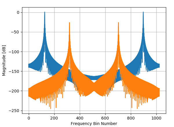
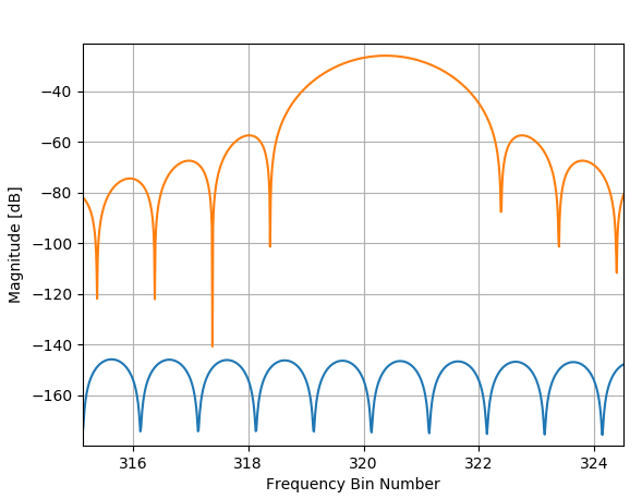
Zooming in on the F2 spectral peak now shows that the leakage from F1 is now over 100 dB lower, but we also see the drawback of windowing- the main lobe of the Kernel is wider leading to reduced frequency selectivity. (The rectangular window has the best selectivity with the narrowest possible main lobe, but the worst dynamic range due to the high sidelobe level and slow roll-off).

Zoom In on F2 Peak Location - With Hann Window Zoom in of Hann
For more info on DTFT vs DFT and approximating the DTFT with zero padding see Getting the DTFT from the DFT samples and For 2D signals can it be said that the frequency response is the same as the Fourier transform?

For additional details on windowing see: Why would one use a Hann or Bartlett window?

For additional details on spectral leakage see: Intuition for sidelobes in FFT

Suggestions for Efficient Processing

Assuming the objective is to only find the magnitudes for each of the tones, if 0.01 dB accuracy is sufficient, a suggestion is to use a flattop window, which provides nearly 100 dB of sidelobe rejection while maintaining a very flat main lobe in frequency extending out to $\pm 0.5$ bins. This means no further interpolation would be necessary to estimate the magnitude of a tone located at a fractional bin frequency to get an estimate within 0.01 dB of the actual magnitude.

Below shows an example of the Kernel (DTFT) of a flattop window with just 128 samples, showing nearly 100 dB of sidelobe rejection reached at a 5 bin offset.
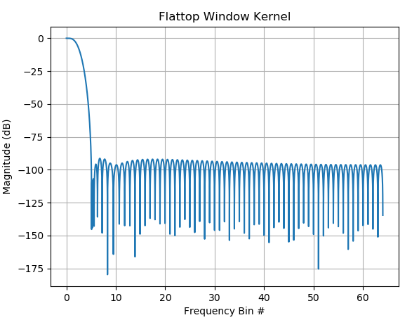
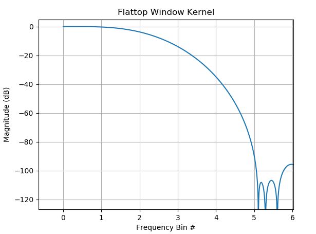
Flat Top Kernel

Zoom in of main lobe

Zooming in to see the flatness, we see that with 128 points we maintain less than 0.01 dB flatness over $\pm 0.5$ bins.
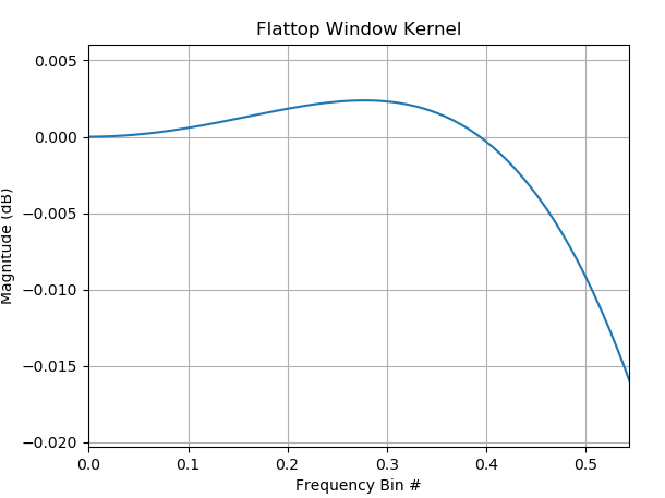
Zoom in showing flatness of main lobe

If the $0.01$ dB magnitude accuracy was acceptable, the solution to minimize processing would be to choose the maximum DFT size required to ensure no two tones are spaced closer than 5 bins based on the minimum tone proximimity (a 58.7 dB leakage which occurs at approximately 4.6 bins would cause a maximum amplitude error of 0.01 dB). This would set the minimum number of samples to process, after which can be multiplied by the flattop window and fft'd where the maximum bins would be sufficient to provide the amplitude estimates.

Here is an interesting paper with further information on designing the flattop window to any passband error specification (at the expense of sidelobe performance), as well as other optimized flattop solutions: Design and Improvement of Flattop Windows with Semi Infinite Optimization.

$\endgroup$
9
  • $\begingroup$ great answer, thank you. I'm aware, frequency estimation accuracy is improved by windowing (leakage is reduced and aliasing between neighbouring peaks too, if they are not too close). E.g. from dft frequency accuracy scales like 1/N and 1/N^2 with hann window. Something similar should hold for amplitudes, but I don't see 1/N^2 if sum in expression for amp is evaluated symbolically, I'll check symbolic solution more carefully later. $\endgroup$
    – I.M.
    Commented Sep 12, 2020 at 5:08
  • $\begingroup$ so, is this method to estimate amplitudes the most appropriate for this problem? $\endgroup$
    – I.M.
    Commented Sep 12, 2020 at 5:11
  • $\begingroup$ the qualitive mechanism that you described is clear. $\endgroup$
    – I.M.
    Commented Sep 12, 2020 at 5:14
  • $\begingroup$ perhaps the problem is with index $n$ in the exponent, it should be replaced with $n-1$. I've also tested Kaiser window and it work great, same for cosine window of different orders. As for spectra interpolation, padding is expensive, I use ffrft and interpolating polynomial bear ffrft maximum $\endgroup$
    – I.M.
    Commented Sep 12, 2020 at 5:36
  • $\begingroup$ Thanks for that link and that makes perfect sense and sounds like a good approach-- you'll find Cedron's blog posts and his work on estimation interesting as well. I don't see an index n in the exponent, are you talking about your summation from 1 to N? typically it is from 0 to N-1, but that shouldn't change the result since it is cyclically invariant over any range (0 to N-1, or 1 to N, or 2 to N+1, etc). $\endgroup$ Commented Sep 12, 2020 at 5:52
2
$\begingroup$

Okay, these results are little worse than I expected. I'm going to have a second look.

Here is the signal generator:

import numpy as np

#=============================================================================
def main():

        N = 64
        
        x = np.zeros( N )

        for n in range( N ):
          x[n] = 1.0    * np.cos( 2 * np.pi * 0.123 * n ) \
               + 0.5    * np.sin( 2 * np.pi * 0.123 * n ) \
               + 0.1    * np.cos( 2 * np.pi * 0.378 * n ) \
               + 0.0001 * np.sin( 2 * np.pi * 0.378 * n ) 

        f = open( "TwoTone.txt", "w" )
        
        for n in range( N ):
          f.write( str( x[n] ) + "\n" )
                       
        f.close()               
                  
#=============================================================================
main()

Here is the 16 point case:

16
Peak at 2  657.100
Peak at 6  65.527

    2   1.967574268   1.127686414  -0.462437761   9.677939450
    6   6.096984210   0.112391665  -0.215513086   8.704864641
theShiftSquareSum 1.18480464437

    2   1.967574268   1.118934768  -0.461595191   0.000064761
    6   6.096984210   0.113199253  -0.209107938   0.047386657
theShiftSquareSum 0.000153884710745

    2   1.967574268   1.118950503  -0.461589923   0.000002945
    6   6.096984210   0.113177001  -0.209377985   0.047165809
theShiftSquareSum 1.11779322854e-07

    2   1.967574268   1.118950601  -0.461589890   0.000002946
    6   6.096984210   0.113177942  -0.209366691   0.047171378
theShiftSquareSum 1.967368058e-10

    2   1.967574268   1.118950602  -0.461589890   0.000002946
    6   6.096984210   0.113177902  -0.209367163   0.047171141
theShiftSquareSum 3.44244306479e-13

    2   1.967574268   1.118950602  -0.461589890   0.000002946
    6   6.096984210   0.113177904  -0.209367144   0.047171151
theShiftSquareSum 6.02574348723e-16

    2   1.968   1.119  -0.462    0.12297    1.00185    0.49835
    6   6.097   0.113  -0.209    0.38106    0.11071    0.02352

Here is the 64 point case:

64
Peak at 8  1596.112
Peak at 24  152.103

    8   7.871922908   1.125979444  -0.458494786  215.881795607
   24  24.200735389   0.108911265  -0.137066216  196.820341835
theShiftSquareSum 1.76424051554

    8   7.871922908   1.118802923  -0.461915642   0.000058885
   24  24.200735389   0.109116108  -0.137631501   0.048358225
theShiftSquareSum 5.61078445351e-05

    8   7.871922908   1.118765771  -0.461961717   0.000005558
   24  24.200735389   0.109117039  -0.137631515   0.048362634
theShiftSquareSum 3.29842827826e-09

    8   7.871922908   1.118765273  -0.461962339   0.000005549
   24  24.200735389   0.109117039  -0.137631515   0.048362634
theShiftSquareSum 5.85271671495e-13

    8   7.871922908   1.118765266  -0.461962348   0.000005549
   24  24.200735389   0.109117039  -0.137631515   0.048362634
theShiftSquareSum 1.06705350002e-16

    8   7.872   1.119  -0.462    0.12300    1.00150    0.49864
   24  24.201   0.109  -0.138    0.37814    0.10809    0.01497

The last three columns should match the parameters. I was expecting accuracy at least to $ 10^{-15} $ in this noiseless case.

$\endgroup$

Your Answer

By clicking “Post Your Answer”, you agree to our terms of service and acknowledge you have read our privacy policy.

Not the answer you're looking for? Browse other questions tagged or ask your own question.