Advice on designing a digital filter that doesn't have phase-sensitive edge artifacts?

Question

I'm pretty well versed in statistics, but not really digital signal filtering. I have a data scenario where I expected to be able to pretty easily filter out some noise (human pulse) that's at a known frequency band, but I'm having a lot of trouble using the standard tools in the scipy.signal library and think I must be misunderstanding how to design digital filters. I have a notebook here that walks through my explorations thus far, but the gist is that the standard scipy filters seem to cause large distortions at the start and end of my signal, with the precise behaviour dependent on the phase of the noise signal I'm trying to subtract. Just in case the above binder link goes down, I'll include some of the key points below as well:

First generating some synthetic data that's similar to my real data:

#generate time vector
samples_per_sec = 10.0
total_time = 40.0
time = np.linspace(0, total_time, int(total_time*samples_per_sec))

#generate the pulse signal
pulse_hz = 1.0
pulse_phase = np.radians(0)
pulse = np.sin(time*(2*np.pi)*pulse_hz - pulse_phase)

#generate the BOLD signal (just something that goes up then down)
dist = stats.beta(2, 2)
bold = dist.pdf((time-10)/20) / 10.0 # division by 10 to make bold a small signal

#combine
pulse_plus_bold = pulse+bold
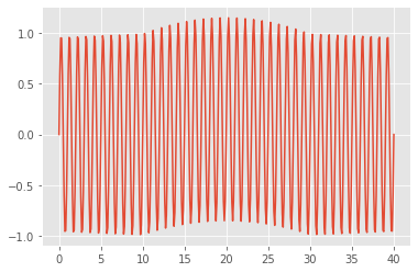
plt.plot(time, pulse_plus_bold);

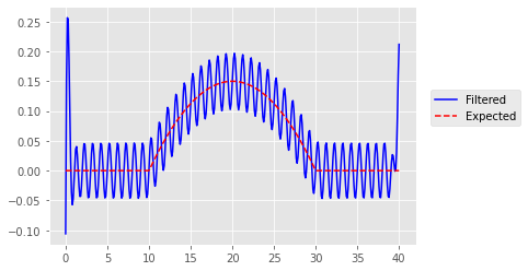
Try a 1st order butterworth:

#1st order butterworth filter in ba mode
ba1 = signal.butter(
    output = 'ba'
    , N = 1 #needs to be low if using output='ba', else use output='sos' and sosfiltfilt
    , Wn = [0.5,1.5]
    , btype = 'bandstop'
    , fs = samples_per_sec
)
filtered_ba1_nopad = signal.filtfilt(
    b = ba1[0]
    , a = ba1[1]
    , x = pulse_plus_bold
    , padtype = None
)
plt.plot(time, filtered_ba1_nopad, 'b');
plt.plot(time, bold, 'r--');
plt.legend(['Filtered', 'Expected'], loc=(1.04,.5));

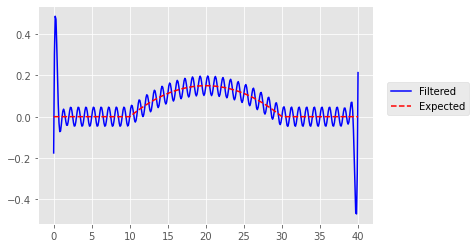
First-order butterworth with even padding:

filtered_ba1_pad_even = signal.filtfilt(
    b = ba1[0]
    , a = ba1[1]
    , x = pulse_plus_bold
    , method = 'pad'
    , padtype = 'even'
)
plt.plot(time, filtered_ba1_pad_even, 'b');
plt.plot(time, bold, 'r--');
plt.legend(['Filtered', 'Expected'], loc=(1.04,.5));

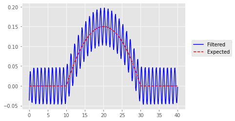
First-order butterworth with odd padding:

filtered_ba1_pad_odd = signal.filtfilt(
    b = ba1[0]
    , a = ba1[1]
    , x = pulse_plus_bold
    , method = 'pad'
    , padtype = 'odd'
)
plt.plot(time, filtered_ba1_pad_odd, 'b');
plt.plot(time, bold, 'r--');
plt.legend(['Filtered', 'Expected'], loc=(1.04,.5));

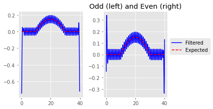
This latter looks really good! But after playing around I discovered that whether odd or even (or either) padding works better seems to be contingent on the phase of the signal being filtered-out. As an example, while the above obtained excellent filtering with odd-padding, here's the same scenario but with a phase-shift added to the pulse signal that yields edge artifacts in both odd and even:

phase = np.radians(45)
pulse_shifted = np.sin(time*(2*np.pi)*pulse_hz - phase)
pulse_shifted_plus_bold = pulse_shifted+bold

filtered_shifted_ba1_pad_odd = signal.filtfilt(
    b = ba1[0]
    , a = ba1[1]
    , x = pulse_shifted_plus_bold
    , method = 'pad'
    , padtype = 'odd'
)
filtered_shifted_ba1_pad_even = signal.filtfilt(
    b = ba1[0]
    , a = ba1[1]
    , x = pulse_shifted_plus_bold
    , method = 'pad'
    , padtype = 'even'
)

fig, axes = plt.subplots(nrows=1, ncols=2, figsize=(5, 3))
axes[0].plot(time, filtered_shifted_ba1_pad_odd, 'b')
axes[0].plot(time, bold, 'r--')
axes[1].plot(time, filtered_shifted_ba1_pad_even, 'b')
axes[1].plot(time, bold, 'r--')
fig.tight_layout()
plt.title('Odd (left) and Even (right)')
plt.legend(['Filtered', 'Expected'], loc=(1.04,.5));

I've also tried the 'gust' padding method as well as higher order filters (using sos of course), and observe the same phase-dependent edge artifacts in everything I've tried. Any tips?

Answer 1

Your basic problem is that filtfilt (and most other linear filtering routines) take filters that are designed for infinitely long time expanses, and apply them to a chunk of data as if the data were extended infinitely in both directions with zeros.

So you have a legitimate bandpass filter, and it's "seeing" a legitimate jump in the signal at the starting point of your signal.

There's three basic approaches you can take; the first two are ad-hoc and easy, the third one is difficult if you're starting from first principles. It's certainly been solved out there someplace, but a brief search here on "filter finite-length data" didn't find me joy.

Approach 1: window the input data

Take your input data, and multiply it by something that'll make it taper off at the ends. I.e. a ramp from 0 to 1 over 10 samples at each end, or $\frac{1}{2}\left (1 - \cos \frac{\pi n}{N} \right)$ for N samples at each end (suitably reversed on the left end). You'll have some artifacts (a rising sine wave isn't the same as a steady one, after all), but they'll be attenuated. Here's python code implementing a cosine edge attenuation with the ability to customize what central % of the signal is kept as 1:

def attenuate_edges(signal,time,edge_attenuation_percent):
  start = int(np.floor(len(time)*edge_attenuation_percent))
  end = int(len(time)-start)
  ramp = (1-np.cos(np.pi*(np.arange(start)/start)))/2
  edge_attenuator = np.ones(len(time))
  edge_attenuator[0:start] = ramp
  edge_attenuator[end:len(time)] = np.flip(ramp)
  return(signal*edge_attenuator)

Approach 2: Trim the output data

Do what you're doing now, and lop off the nastiness at the ends. This is probably the easiest, and if you can just collect a bit more data, doesn't lose you anything.

Approach 3: Do a proper estimate of the interfering signal, and subtract it out

This will be fun-fun if you love math and have the time. Basically you'll use the fact that the value of your interfering signal at time $n$ correlates in a specific way with the values of your interfering signal at time $k$ for all values of $n$ and $k$ in your data set. You'll probably end up with something that looks a lot like a Wiener or a Kalman filter, that takes the end-effects into account. Your estimate will be worse at the ends, but this will show up as a bit of noise on the ends -- not as those honkin' big pulses.

If I couldn't figure out the search terms for this, it would take me a day to do and another day to verify, and supposedly an expert. OTOH, Gauss or Laplace probably invented it in the 19th century, and may even have thought it important enough to write down, somewhere. So I'm sure the method exists.