What is the relationship between image spatial domain and FFT powerspectrum?

Question

I am trying to perform contrast-transfer-function for pictures which were recorded in defocus. To do so, I have to calculate the contrast-transfer function from the Thon rings and fit the function to 1D radial average of the spectrum. Let's say that I have a picture in spatial domain where single pixel is 1.7 Angstrom size, which gives me a Nyquist Limit of resolution 2*1.7 A. So I know, that the resolution limit in my powerspectrum will be 1 / 2*1.7A. How can I connect the radial average from powerspectrum with the resolution? That is the relation of each pixel in the spectrum to resolution? I would be very grateful for some hints! Thanks!

Answer 1

The Contrast Transfer Function (CTF) is essentially equivalent to the frequency response of your system.

Therefore, your question is about how to read the two dimensional Discrete Fourier Transform and how to interpret its content.

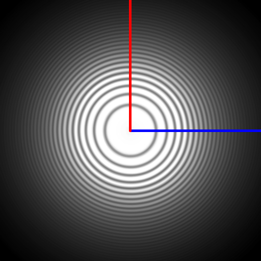
To relate what is mentioned in that answer to your specific question, consider the following CTF, obtained from Wikipedia (Axis added by me):

This is a two dimensional spectrum. If you are familiar with a one dimensional spectrum, it is as if you took that one and rotated it about the centre of the image.

Therefore, low (spatial) frequencies are towards the centre of the image and high (spatial) frequencies are towards the edges of the image.

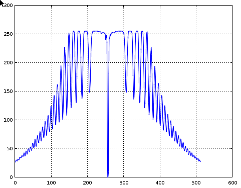
In fact, if we take a cross section of that image (along the direction of the blue line), we see something like this:

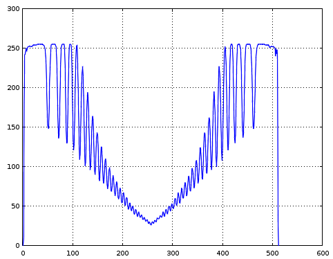
And if we shift the origin of the spectrum to its conventional position (for a 1D spectrum), we get:

So, this now describes how well each spatial frequency goes through the optical system assuming, it is symmetrical.

To relate this to physical frequency, we have to do a bit more work. Now, this is a simple grayscale image, which means that its maximum value is 255. So to normalise the "height" of this curve, we need to simply divide by 255.

The other thing we have to do is to normalise the frequency. This image is 512x512, the DC (or, constant value) is at 0, the Fs is at 512 and the Nyquist frequency is at 256. The formula is a plain simple division of $f = \frac{k}{XDim} \cdot Fs$ where $k$ is the frequency "bin" (of the discrete spectrum) and the fractional part of this we can simply represent in the graph.

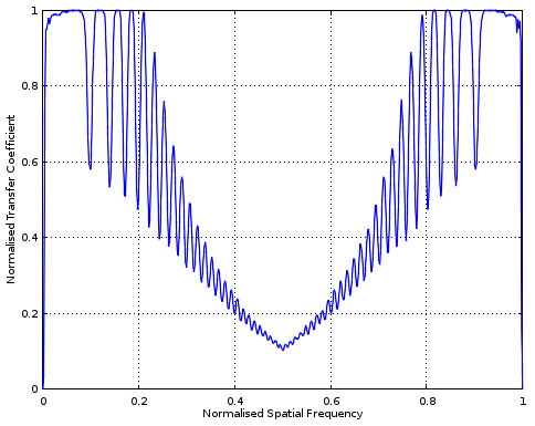
Taking all of this into account gives us:

So, now, whatever your Fs turns out to be, you can put it on the diagram and work backwards to find how much each spatial frequency gets diminished as it passes through this system.

Spatial resolution is measured in "lines" per unit of length. In your case, your pixel size is 1.7Å. The "highest" frequency (in any direction) that can theoretically go through a system that is digitised at that level is one black line of width 1.7Å followed immediately by another white line of width 1.7Å and that is one cycle of period 3.4Å.

Therefore, your Nyquist frequency is 1 line per 3.4Å or $\approx 2941176471$ lines per mm.

Hope this helps.

EDIT:

All the plots in this post were created using Octave and the following code:

% Load the image processing package
pkg load image
% Load the image that was downloaded from Wikipedia
I = imread("~/Downloads/CTF.jpg");
% The image is 512x512, let's take the cross section of the image to see a slice of the spectrum
plot(I(256,:));
% Now shift the origin using fftshift
plot(fftshift(I(256,:)));
% Add normalised X and Y axis, labels, grid, etc
plot((0:511)./512,double(fftshift(I(256,:)))/255.0);xlabel("Normalised Spatial Frequency");ylabel("Normalised Transfer Coefficient");grid on;