Convolution of BPSK signal in frequency domain implementation

Question

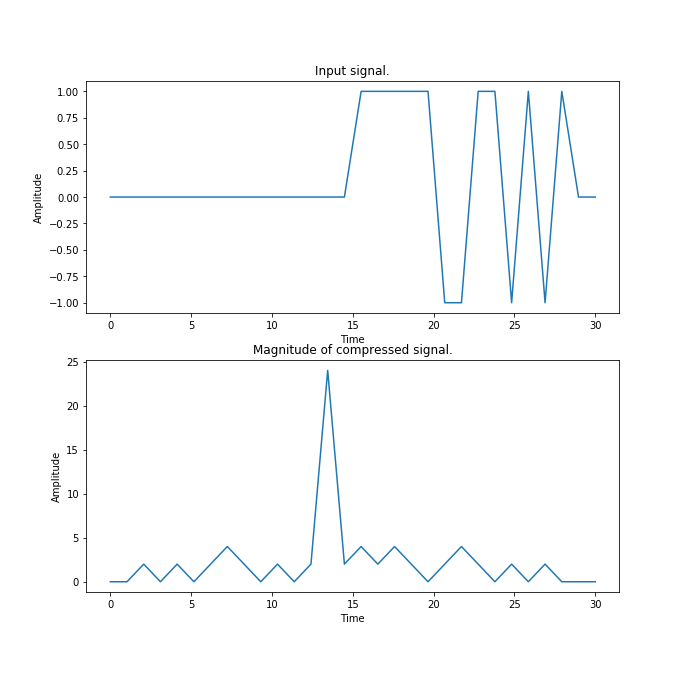
Here is the simplified version of code which implement convolution of BPSK-signal in frequency domain:

import numpy as np
import matplotlib.pyplot as plt
import scipy.fftpack

# Signal and related data.
pulse_code              = "+++++--++-+-+"
pulse_shift             = len (pulse_code) * 1 + 2; # Feel free to move the signal.
sample_number           = len (pulse_code) * 2 + 4; # Feel free to change it.
time                    = np.linspace (0, sample_number, sample_number);
signal_i                = np.zeros (time.size);
signal_q                = np.zeros (time.size);
filter_i                = np.zeros (time.size);
filter_q                = np.zeros (time.size);

# Create signal.
for i in range (time.size):
    if i >= pulse_shift and i < pulse_shift + len (pulse_code):
        m = 1. if pulse_code [i - pulse_shift] == '+' else -1.
        signal_i [i] = m
        signal_q [i] = m

# Create filter.
for i in range (time.size):
    if i < len (pulse_code):
        m = 1. if pulse_code [i - 1] == '+' else -1.
        filter_i [time.size - i - 1] = m
        filter_q [time.size - i - 1] = m

# Prepare to next computation.
signal_complex= signal_i + 1j * signal_q
filter_complex= filter_i + 1j * filter_q

# Go to frequency domain.
spectrum_signal         = scipy.fftpack.fft (signal_complex);
spectrum_filter         = scipy.fftpack.fft (filter_complex);
# Convolution.
spectrum_compressed     = spectrum_signal * spectrum_filter
# Return to time domain.
signal_compressed       = scipy.fftpack.ifft (spectrum_compressed)
# Get envelope.
magnitude_compressed    = np.zeros (time.size)
for i in range (signal_compressed.size):
    magnitude_compressed [i] = np.sqrt (signal_compressed [i].real ** 2 + signal_compressed [i].imag ** 2)

# Print result.
fig = plt.figure ()

plt.subplot (2, 1, 1)
plt.plot (time,  signal_i);
plt.title ("Input signal.")
plt.xlabel ("Time")
plt.ylabel ("Amplitude")

plt.subplot (2, 1, 2)
plt.plot (time, magnitude_compressed);
plt.title ("Magnitude of compressed signal.")
plt.xlabel ("Time")
plt.ylabel ("Amplitude")

plt.show() 

The implementation in my opinion is straightforward and clear, but result which I get is wrong: the maximum sidelobe level is 2 instead of 1, the main lobe is shifted to left and sidelobes aren't symmetric. Can anybody explain where is my error?

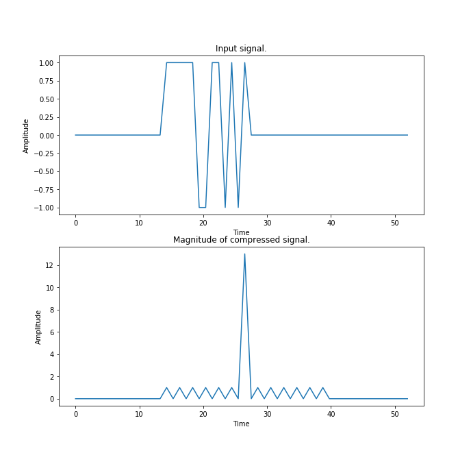
UPD

import numpy as np
import matplotlib.pyplot as plt
import scipy.fftpack

# Signal and related data.
# *_t - time domain;
# *_f - frequency domain.
pulse_code      = "+++++--++-+-+"
N               = 64
M               = len (pulse_code)
L               = N - M + 1
sample_number   = L * 1;
time            = np.linspace (0, sample_number, sample_number);
pulse_shift     = len (pulse_code) + 1;
signal_t        = np.zeros (sample_number) + 1j * np.zeros (sample_number)
filter_t        = np.zeros (N) + 1j * np.zeros (N)
chunk_t         = np.zeros (N) + 1j * np.zeros (N)
chunk_f         = np.zeros (N) + 1j * np.zeros (N)
envelope        = np.zeros (sample_number)

# Create signal.
for i in range (sample_number):
    if i >= pulse_shift and i < pulse_shift + len (pulse_code):
        m = 1. if pulse_code [i - pulse_shift] == '+' else -1.
        signal_t [i] = m + 1j * 0

# Create filter as inverse signal with zero padding.
n = len (pulse_code) - 1
for i in range (len (pulse_code) ):
    m = 1. if pulse_code [len (pulse_code) - i - 1] == '+' else -1.
    filter_t [i] = m + 1j * 0
# and get it's FFT.
filter_f = scipy.fftpack.fft (filter_t)

# Performs convolution using overlap-save method.
for i in range (sample_number / L):
    for j in range (M - 1):
        chunk_t [j] = chunk_t [L + j]
    for j in range (L):
        chunk_t [M - 1 + j] = signal_t [i * L + j]
    chunk_f = scipy.fftpack.fft (chunk_t)
    chunk_f = scipy.fftpack.ifft (chunk_f * filter_f)
    for j in range (L):
        envelope [i * L + j] = np.abs (chunk_f [M - 1 + j])

# Print result.
fig = plt.figure ()

plt.subplot (2, 1, 1)
plt.plot (time,  signal_t);
plt.title ("Input signal.")
plt.xlabel ("Time")
plt.ylabel ("Amplitude")

plt.subplot (2, 1, 2)
plt.plot (time, envelope);
plt.title ("Magnitude of compressed signal.")
plt.xlabel ("Time")
plt.ylabel ("Amplitude")

plt.show()

Answer 1

You're doing a circular convolution where you want a linear convolution.

The Wikipedia article in fast convolution / save-add method has a pretty good explanation of the correct algorithm. Basically, you forgot to zero pad, extract the "valid" part and save the "tail" for the next convolution.

Other than that, your filter is questionable at best, and your method of bpsk generation is unusual in its effects on constellation rotation and power. That's no problem per se, but makes your implementation hard to compare to existing convolution and fast convolution implementations.