10
$\begingroup$

So, I was reading the paper on SURF (Bay, Ess, Tuytelaars, Van Gool: Speeded-Up Robust Features (SURF)) and I can not comprehend this paragraph below:

Due to the use of box filters and integral images, we do not have to iteratively apply the same filter to the output of a previously filtered layer, but instead can apply box filters of any size at exactly the same speed directly on the original image and even in parallel (although the latter is not exploited here). Therefore, the scale space is analysed by up-scaling the filter size rather than iteratively reducing the image size, figure 4.

This is figure 4 in question.
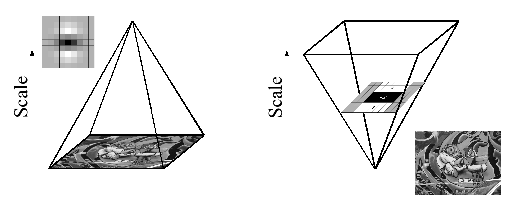
Figure 4

PS: The paper has an explanation of integral image, however the whole content of the paper is based on the particular paragraph above. If anybody has read this paper, can you briefly mention what is going on here. The whole mathematical explanation is quite intricate to have a good grasp first up, so I need some assistance. Thanks.

Edit,couple of issues:

1.

Each octave is subdivided into a constant number of scale levels. Due to the discrete nature of integral images, the minimum scale difference between 2 subsequent scales depends on the length lo of the positive or negative lobes of the partial second order derivative in the direction of derivation (x or y), which is set to a third of the filter size length. For the 9x9 filter, this length lo is 3. For two successive levels, we must increase this size by a minimum of 2 pixels (one pixel on every side) in order to keep the size uneven and thus ensure the presence of the central pixel. This results in a total increase of the mask size by 6 pixels (see figure 5).

Figure 5
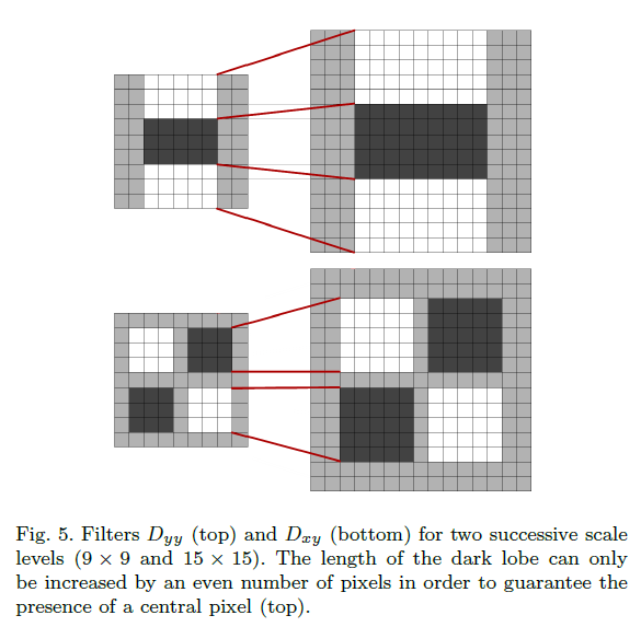
Figure 5

I could not make sense of the lines in the given context.

For two successive levels, we must increase this size by a minimum of 2 pixels (one pixel on every side) in order to keep the size uneven and thus ensure the presence of the central pixel.

I know they are trying to do something with the length of the image, if its even they are trying to make it odd, so that there is a central pixel which will enable them to calculate the maximum or the minimum of the pixel gradient. I am bit iffy about its contextual meaning.

2.

In order to calculate descriptor Haar wavelet is used.
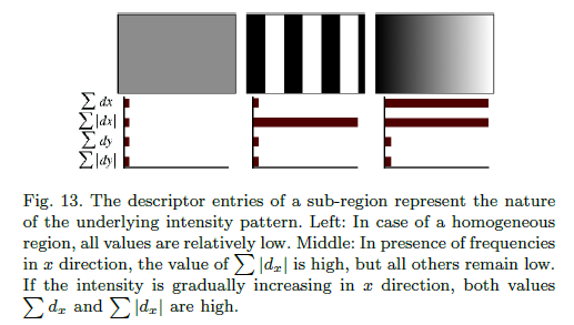
Haar Wavelet

How is the middle region has low $\sum\ dx$ but high $\sum\ |dx|$.

3.
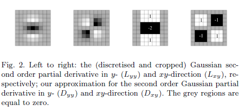
Another one

What is the necessity of having an approximate filter?

4. I have no issue with the way that they found out the size of the filter. They "did" something empirically. However, I have some nagging issue with this piece of line

The output of the 9x9 filter, introduced in the previous section, is considered as the initial scale layer, to which we will refer as scale s = 1.2 (approximating Gaussian derivatives with σ= 1.2).

How did they found out about the value of σ . Moreover how does the calculation of scaling done shown in the image below.The reason I am stating about this image is that the value of s=1.2 keeps on recurring, without clearly stating about its origin. Scale Image
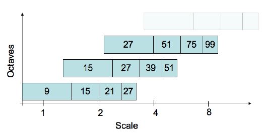
5. The Hessian Matrix represented in terms of L which is the convolution of second order gradient of Gausssian filter and the image.

However the "approximated" determinant is said to contain only terms involving second order Gaussian filter.

The value of w is:

My question why the determinant is calculated like that above, and what is the relationship between approximate Hessian and Hessian matrix.

$\endgroup$
8
  • $\begingroup$ Hey! I added the author names and article title in your questions, I hope you don't mind. First, it makes the article searchable even if the link goes dead. Second, as somebody who does research, I think crediting authors with their names and names of the publication is the least we can do to acknowledge their work :) $\endgroup$
    – penelope
    Commented Jan 6, 2014 at 16:23
  • $\begingroup$ @penelope: I was half scared that people would down-vote me to oblivion. $\endgroup$
    – motiur
    Commented Jan 6, 2014 at 16:25
  • $\begingroup$ I think it's a really nice question, one of the more interesting ones recently. I never got into SURF myself, but I might try and take a look tomorrow and see if I can contribute, the question actually made me interested :) and PS: if you're doing this as a part of an "official" Uni project, I'm sure your supervisor would gladly help you (especially if you're at Master level). A part of their job is to teach you how to read scientific literature. $\endgroup$
    – penelope
    Commented Jan 6, 2014 at 16:28
  • $\begingroup$ PPS: you might want to edit your question to add a short explanation of the terms integral image and box filter: understanding what you understand will probably help us understand what you don't understand ;) $\endgroup$
    – penelope
    Commented Jan 6, 2014 at 16:29
  • $\begingroup$ @penelope: You are a pretty nice girl/guy, whatever. And no I have to have a literature review of this paper, I read the one written by David Lowe both 2004 and 1999. That one was quite understable, plus there was a nice youtube lecture on that. The problem is there is tons of mathematical terms used in this paper, the one with SURF. If you don't have a mathematical model in your head, its tricky to see the main idea. $\endgroup$
    – motiur
    Commented Jan 6, 2014 at 16:35

2 Answers 2

11
$\begingroup$

What's SURF?

In order to correctly understand what is going on, you also need to be familiar with SIFT: SURF is basically an approximation of SIFT. Now, the real question becomes: what's SIFT?.

SIFT is both a keypoint detector and a keypoint descriptor. In the detector part, SIFT is essentially a multi-scale variant of classical corner detectors such as the Harris corner, and that has the ability to auto-tune the scale. Then, given a location and a patch size (derived from the scale), it can compute the descriptor part.

SIFT is very good at matching locally affine pieces of images, but it has one drawback: it is expensive (i.e., long) to compute. A large amount of time is spent in computing the Gaussian scale-space (in the detector part), then in computing histograms of the gradient direction (for the descriptor part).

Both SIFT and SURF can be seen as difference of Gaussians with automatic scale (i.e., Gaussian sizes) selection. This, you construct first a scale-space where the input image is filtered at different scales. The scale-space can be seen as a pyramid, where two consecutive images are related by a scale change (i.e., the size of the Gaussian low-pass fiéter has changed), and scales are then grouped by octaves (i.e., a big change in the size of the Gaussian filter).

  • In SIFT, this is done by repeatedly filtering the input with a Gaussian of fixed width until the scale of the next octave is reached.
  • In SURF, you do not suffer any runtime penalty from the size of the Gaussian filter thanks to the use of the integral image trick. Thus, you compute directly the image filtered at each scale (without using the result at the previous scale).

The approximation part

Since computing the Gaussian scale-space and the histograms of the gradient direction is long, it is a good idea (chosen by the authors of SURF) to replace these computations by fast approximations.

The authors remarked that small Gaussians (like the ones used in SIFT) could be well approximated by square integrals (also known as box blur). These rectangle averages have the nice property to be very fast to obtain thanks to the integral image trick.

Furthermore, the Gaussian scale-space is actually not used per se, but to approximate a Laplacian of Gaussians (you can find this in the SIFT paper). Thus, you do not need just Gaussian-blurred images, but derivatives and differences of them. So, you just push a bit further the idea of approximating a Gaussian by a box: first derive a Gaussian as many times as needed, then approximate each lobe by a box of the correct size. You will eventually end up with a set of Haar features.

Increment by 2

This is just an implementation artifact, as you have guessed. The goal is to have a central pixel. The feature descriptor is computed with respect to the center of the image patch to be described.

Middle region

When going from a black ray to a white ray, you have something like $\sum_{\text{all pix in column}} \partial x = A$. Then, going from white to black, you have the opposite sum: $\sum_{\text{all pix in column}} \partial x = -A$. Thus, you have a small $\sum \partial x$ for the window, but a higher sum of the magnitudes.

Magic number

The first scale is obtained by applying a blur with $\sigma = 1.2$ (or 1.4 in some papers). This is because a natural (real) sharp image can be considered as being the result of the convolution of an ideal (without aliasing) image with a blur kernel of width $\sigma = 1.2$. I can't really remember where it comes from, but it was also explicitly studied in Guoshen Yu's work on A-SIFT, so you might check this page.

$\endgroup$
16
  • $\begingroup$ Thanks for the explanation, it cleared some of the stuff, let me see whether anybody has a more elaborate understanding. $\endgroup$
    – motiur
    Commented Jan 6, 2014 at 17:01
  • $\begingroup$ I've edited the answer with respect to your new questions. $\endgroup$
    – sansuiso
    Commented Jan 8, 2014 at 7:16
  • $\begingroup$ Oh yeah thanks, appreciable. The paper is kind a long, so lots of thing goes at once. $\endgroup$
    – motiur
    Commented Jan 8, 2014 at 9:38
  • $\begingroup$ Care to see my latest edit? $\endgroup$
    – motiur
    Commented Jan 8, 2014 at 13:18
  • 1
    $\begingroup$ It's a mix of common shared knowledge (small Gaussians are well approximated by box blurs), experimentation (min/max sizes of objects of interest in real world images) and mathematics (given an initial patch size, computing rectangles and Gaussians that fit into). $\endgroup$
    – sansuiso
    Commented Jan 8, 2014 at 14:57
5
$\begingroup$

In order to identify the potential interest points, difference-of-Gaussian function (DOG) is often used to process the image, thus making it invariant to scale and orientation.

In SIFT, image pyramids are established by filtering each layer with DOG of increasing sigma values and taking the difference.

On the other hand, SURF applies a much faster approximation of second-order Gaussian partial derivatives with Laplacian of Gaussian (LoG) and the square filters of different size (9*9, 15*15, ...). The computational cost is independent of the filter size. There is no down-sampling (change sigma) for higher levels in the pyramid, but only the up-scale of filter size resulting in having images of the same resolution.

EDIT

One additional note: the authors in your paper further simplify the Gaussian second derivative at the 4 orientations (x,y,xy,yx) with the kernel [1 -2 1], [1 -2 1]', [1 -1;-1 1], and [-1 1;1 -1]. When the filter size increases, you just need to extend the simplified kernel regions to achieve the larger one. And it is equivalent to the DOG with different scales (LoG curve is the same shape as DOG, and the filter size makes their width also equal).

$\endgroup$

Your Answer

By clicking “Post Your Answer”, you agree to our terms of service and acknowledge you have read our privacy policy.

Not the answer you're looking for? Browse other questions tagged or ask your own question.