"Low-pass filter" in non-EE, software API contexts

Question

I am an experienced software engineer and am working on smartphone sensors. I've taken fundamental EE classes in DSP and am trying to apply my knowledge. I believe that I understand convolution, transfer functions, z-transform, etc. I know a little bit about FIR and IIR filters.

Now, when reading through software APIs and documentation, I see people are applying a LPF to sensor data in the time domain. I know that you do that through the use of difference equations (e.g. y[i] = y[i-1] + 2*x[i]), but I learned in my EE class that LPF are typically applied through the convolution operation where you convolve the time signal with the coefficients of a sinc wave (for example) and with a specific cut-off frequency. So the colloquial use of "low-pass filter" is not exact enough for me.

For example, the Google Android API has this documentation: http://developer.android.com/reference/android/hardware/SensorEvent.html#values

 public void onSensorChanged(SensorEvent event)
 {
      // alpha is calculated as t / (t + dT)
      // with t, the low-pass filter's time-constant
      // and dT, the event delivery rate

      final float alpha = 0.8;

      gravity[0] = alpha * gravity[0] + (1 - alpha) * event.values[0];
      gravity[1] = alpha * gravity[1] + (1 - alpha) * event.values[1];
      gravity[2] = alpha * gravity[2] + (1 - alpha) * event.values[2];

      linear_acceleration[0] = event.values[0] - gravity[0];
      linear_acceleration[1] = event.values[1] - gravity[1];
      linear_acceleration[2] = event.values[2] - gravity[2];
 }

How do I interpret that low-pass filter? What is the cut-off frequency? What is the transition bandwidth? Are they using this LPF solely to do averaging?

Answer 1

The filter in your example is a first-order infinite impulse response (IIR) filter. Its transfer function is:

$$ H(z) = \frac{1 - \alpha}{1 - \alpha z^{-1}} $$

which corresponds to a difference equation of:

$$ y[n] = \alpha y[n-1] + (1-\alpha) x[n] $$

where $x[n]$ is the filter input and $y[n]$ is the filter output.

This type of filter is often used as a low-complexity lowpass filter and is often called a leaky integrator. It is favored because of its simple implementation, low computational complexity, and its tunability: its cutoff frequency depends upon the value of $\alpha$. $\alpha$ can take on values on the interval $[0,1)$. $\alpha = 0$ yields no filtering at all (the output is equal to the input); as $\alpha$ increases, the cutoff frequency of the filter decreases. You can think of $\alpha = 1$ as a boundary case where the cutoff frequency is infinitely low (the filter output is zero for all time).

You can think of this intuitively by noticing that the filter input is weighted by $\alpha$, so as the parameter increases, the quantity $1-\alpha$ decreases, so each input sample has a smaller proportional effect on the value of any particular output sample. This has the effect of smearing out the filter's impulse response over a longer period of time. Summing over a longer period of time is similar to computing a long moving average. As the length of a moving average increases, the cutoff frequency of the average decreases.

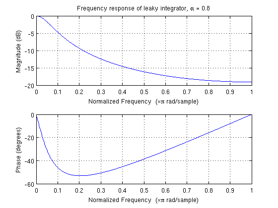
For your example, where $\alpha = 0.8$, the frequency response of the filter is as follows:

From the example, I would guess that this filter is being used to smooth high-frequency noise out of a time series of measurements from a sensor, trying to tease out a comparatively low-frequency signal of interest. This would be a very typical application for this sort of filter.

On your other sub-question, you are correct that filtering is often implemented via convolution of the input signal with the filter's impulse response. In most cases, this is only done with finite impulse response (FIR) filters. IIR filters such as this one are typically implemented using the filter's difference equation; since an IIR system's impulse response is infinitely long, you must truncate it to some finite length to make convolution with it tractable, at which point the filter is no longer IIR. The difference equation format is almost always cheaper to implement computationally, although the feedback inherent in that structure can lead to numerical issues that must be addressed (such as internal overflow and roundoff error accumulation).

Answer 2

To summarize, IIR filters based on simple idealized physical models, such as an RC filter, have a small number of poles and zeros, and thus are usually implemented as a difference equation, as a small number of poles or zeros implies very few arithmetic operations per sample using a difference equation.

As an IIR implies an infinite length impulse response, convolution would either require forever to compute, or the use of an approximation.

FIR filters are usually implemented by convolution with the finite length impulse response (or by FFT fast convolution if the filter is long enough for that to be computationally efficient). These kinds of filters are more often used when one can approximate a desired frequency response specification with an finite length impulse response, rather than knowing where the Z-plane poles and zeros might be located.

However since a filter with a sharp specification implies a long FIR convolution, the implementation of FIR filters can a lot slower, and the setup may involve many more lines of code, which may be why FIR filters might not be used as often in simple software examples.

Answer 3

I find myself coming back to this post time and time again. Thank you for asking the question. Here is a great, computationally-friendly implementation of the leaky integrator in C (intended for a microcontroller).

First, some rearrangement: y = α * x + (1 − α) * y_last = α * (x - y_last) + y_last

if we restrict α to be about 12%, 25%, 50%, (1/8, 1/4, 1/2,...). We can take advantage of some efficient bit-shifting. Taking the case of 1/8, 8 => 2^3 => (downshift 3 times)

= (x - y_last) / 8 + y_last

#define SMOOTHING_FACTOR       (3)

int16_t FilterSample(int16_t new_sample)
{
  static int16_t last_result = 0;

  // Each bit shift down is equivalent to dividing-by-two
  last_result = (new_sample - last_result) >> SMOOTHING_FACTOR) + last_result;

  return last_result;
}

Hope it helps.