fixed typos, clarified difference equation
Source Link
Jason R
  • 24.8k
  • 2
  • 70
  • 74

The filter in your example is a first-order infinite impulse response (IIR) filter. Its difference equationtransfer function is:

$$ H(z) = \frac{1 - \alpha}{1 - \alpha z^{-1}} $$

which corresponds to a difference equation of:

$$ y[n] = \alpha y[n-1] + (1-\alpha) x[n] $$

where $x[n]$ is the filter input and $y[n]$ is the filter output.

This type of filter is often used as a low-complexity lowpass filter and is often called a leaky integrator. It is favored because of its simple implementation, low computational complexity, and its tunability: its cutoff frequency depends upon the value of $\alpha$. $\alpha$ can take on values on the interval $[0,1)$. $\alpha = 0$ yields no filtering at all (the output is equal to the input); as $\alpha$ increases, the cutoff frequency of the filter decreases. You can think of $\alpha = 1$ as a boundary case where the cutoff frequency is infinitely low (the filter output is zero for all time).

You can think of this intuitively by noticing that the filter input is weighted by $\alpha$, so as the parameter increases, the quantity $1-\alpha$ decreases, so each input sample has a smaller proportional effect on the value of any particular output sample. This has the effect of smearing out the filter's impulse response over a longer period of time. Summing over a longer period of time is similar to computing a long moving average. As the length of a moving average increases, the cutoff frequency of the average decreases.

For your example, where $\alpha = 0.8$, the frequency response of the filter is as follows: enter image description here
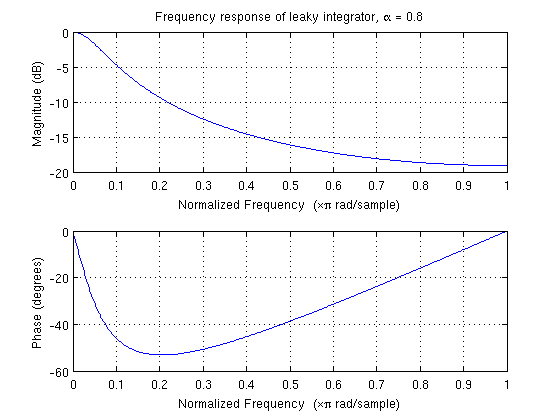
From the example, I would guess that this filter is being used to smooth high-frequency noise out of a time series of measurements from a sensor, trying to tease out a comparatively low-frequency signal of interest. This would be a very typical application for this sort of filter.

On your other sub-question, you are correct that filtering is often implemented via convolution of the input signal with the filter's impulse response. In most cases, this is only done with finite impulse response (FIR) filters. IIR filters such as this one are typically implemented using the filter's difference equation; since an IIR system's impulse response is infinitely long, you must truncate it to some finite length to make convolution with it tractable, at which point the filter is no longer IIR. The difference equation format is almost always cheaper to implement computationally, although the feedback inherent in that structure can lead to numerical issues that must be addressed (such as internal overflow and roundoff error accumulation).

The filter in your example is a first-order infinite impulse response (IIR) filter. Its difference equation is:

$$ H(z) = \frac{1 - \alpha}{1 - \alpha z^{-1}} $$

This type of filter is often used as a low-complexity lowpass filter and is often called a leaky integrator. It is favored because of its simple implementation, low computational complexity, and its tunability: its cutoff frequency depends upon the value of $\alpha$. $\alpha$ can take on values on the interval $[0,1)$. $\alpha = 0$ yields no filtering at all (the output is equal to the input); as $\alpha$ increases, the cutoff frequency of the filter decreases. You can think of $\alpha = 1$ as a boundary case where the cutoff frequency is infinitely low (the filter output is zero for all time).

You can think of this intuitively by noticing that the filter input is weighted by $\alpha$, so as the parameter increases, the quantity $1-\alpha$ decreases, so each input sample has a smaller proportional effect on the value of any particular output sample. This has the effect of smearing out the filter's impulse response over a longer period of time. Summing over a longer period of time is similar to computing a long moving average. As the length of a moving average increases, the cutoff frequency of the average decreases.

For your example, where $\alpha = 0.8$, the frequency response of the filter is as follows: enter image description here

From the example, I would guess that this filter is being used to smooth high-frequency noise out of a time series of measurements from a sensor, trying to tease out a comparatively low-frequency signal of interest. This would be a very typical application for this sort of filter.

On your other sub-question, you are correct that filtering is often implemented via convolution of the input signal with the filter's impulse response. In most cases, this is only done with finite impulse response (FIR) filters. IIR filters such as this one are typically implemented using the filter's difference equation; since an IIR system's impulse response is infinitely long, you must truncate it to some finite length to make convolution with it tractable, at which point the filter is no longer IIR. The difference equation format is almost always cheaper to implement computationally, although the feedback inherent in that structure can lead to numerical issues that must be addressed (such as internal overflow and roundoff error accumulation).

The filter in your example is a first-order infinite impulse response (IIR) filter. Its transfer function is:

$$ H(z) = \frac{1 - \alpha}{1 - \alpha z^{-1}} $$

which corresponds to a difference equation of:

$$ y[n] = \alpha y[n-1] + (1-\alpha) x[n] $$

where $x[n]$ is the filter input and $y[n]$ is the filter output.

This type of filter is often used as a low-complexity lowpass filter and is often called a leaky integrator. It is favored because of its simple implementation, low computational complexity, and its tunability: its cutoff frequency depends upon the value of $\alpha$. $\alpha$ can take on values on the interval $[0,1)$. $\alpha = 0$ yields no filtering at all (the output is equal to the input); as $\alpha$ increases, the cutoff frequency of the filter decreases. You can think of $\alpha = 1$ as a boundary case where the cutoff frequency is infinitely low (the filter output is zero for all time).

You can think of this intuitively by noticing that the filter input is weighted by $\alpha$, so as the parameter increases, the quantity $1-\alpha$ decreases, so each input sample has a smaller proportional effect on the value of any particular output sample. This has the effect of smearing out the filter's impulse response over a longer period of time. Summing over a longer period of time is similar to computing a long moving average. As the length of a moving average increases, the cutoff frequency of the average decreases.

For your example, where $\alpha = 0.8$, the frequency response of the filter is as follows: enter image description here

From the example, I would guess that this filter is being used to smooth high-frequency noise out of a time series of measurements from a sensor, trying to tease out a comparatively low-frequency signal of interest. This would be a very typical application for this sort of filter.

On your other sub-question, you are correct that filtering is often implemented via convolution of the input signal with the filter's impulse response. In most cases, this is only done with finite impulse response (FIR) filters. IIR filters such as this one are typically implemented using the filter's difference equation; since an IIR system's impulse response is infinitely long, you must truncate it to some finite length to make convolution with it tractable, at which point the filter is no longer IIR. The difference equation format is almost always cheaper to implement computationally, although the feedback inherent in that structure can lead to numerical issues that must be addressed (such as internal overflow and roundoff error accumulation).

Source Link
Jason R
  • 24.8k
  • 2
  • 70
  • 74

The filter in your example is a first-order infinite impulse response (IIR) filter. Its difference equation is:

$$ H(z) = \frac{1 - \alpha}{1 - \alpha z^{-1}} $$

This type of filter is often used as a low-complexity lowpass filter and is often called a leaky integrator. It is favored because of its simple implementation, low computational complexity, and its tunability: its cutoff frequency depends upon the value of $\alpha$. $\alpha$ can take on values on the interval $[0,1)$. $\alpha = 0$ yields no filtering at all (the output is equal to the input); as $\alpha$ increases, the cutoff frequency of the filter decreases. You can think of $\alpha = 1$ as a boundary case where the cutoff frequency is infinitely low (the filter output is zero for all time).

You can think of this intuitively by noticing that the filter input is weighted by $\alpha$, so as the parameter increases, the quantity $1-\alpha$ decreases, so each input sample has a smaller proportional effect on the value of any particular output sample. This has the effect of smearing out the filter's impulse response over a longer period of time. Summing over a longer period of time is similar to computing a long moving average. As the length of a moving average increases, the cutoff frequency of the average decreases.

For your example, where $\alpha = 0.8$, the frequency response of the filter is as follows: enter image description here

From the example, I would guess that this filter is being used to smooth high-frequency noise out of a time series of measurements from a sensor, trying to tease out a comparatively low-frequency signal of interest. This would be a very typical application for this sort of filter.

On your other sub-question, you are correct that filtering is often implemented via convolution of the input signal with the filter's impulse response. In most cases, this is only done with finite impulse response (FIR) filters. IIR filters such as this one are typically implemented using the filter's difference equation; since an IIR system's impulse response is infinitely long, you must truncate it to some finite length to make convolution with it tractable, at which point the filter is no longer IIR. The difference equation format is almost always cheaper to implement computationally, although the feedback inherent in that structure can lead to numerical issues that must be addressed (such as internal overflow and roundoff error accumulation).