Periodogram (Welch) has different levels depending on length of segment/ resolution

Question

I am trying to compute the PSD of a signal in MATLAB using Welch's periodogram method as shown in the code snippet below.

sine = dsp.SineWave('Amplitude',1,'Frequency',10e6,'SampleRate',fs,'SamplesPerFrame',1000000);
y = sine();

nsc = 500000; % 5000 50000
nov = floor(nsc/2);
nff = max(256,2^nextpow2(nsc));

[pxx, f] = pwelch(y,hann(nsc),nov,nff,fs);
pxx = 10*log10(pxx) + 30; % also convert to dBm
plot(f, pxx);

grid on;
xlim([0 20e6]);
xlabel("Frequency (Hz)");
ylabel("PSD (dBm/Hz)");

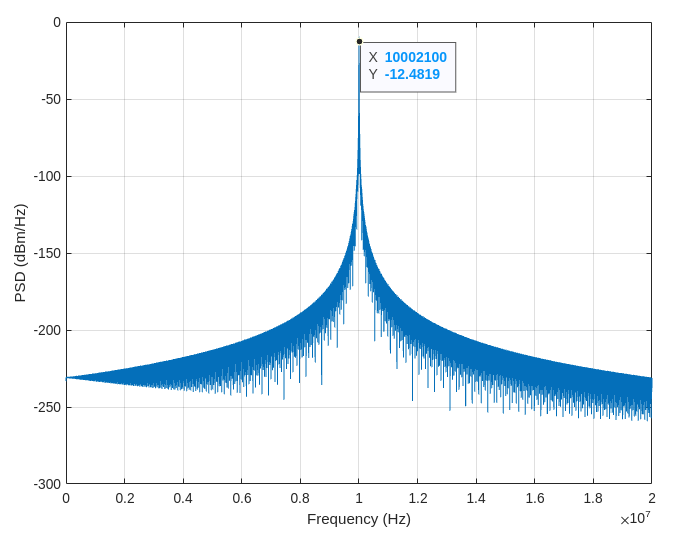
However I get very different power levels depending on the length of the section of data I use which is related to the resolution as shown in the images for $nsc = 5000$ and $50000$ respectively:

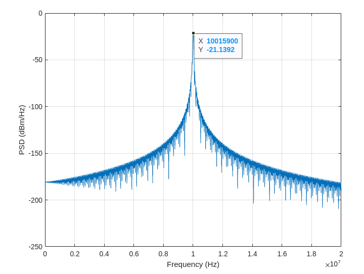
It's very similar to what happens when I use the spectrum analyser and use different resolution bandwidth. With the SA, I typically normalise by subtracting 10log10(RBW).

How should I go about making the PSD from the MATLAB code more consistent? Subtracting $10log_{10}(fs/nsc)$ doesn't seem to be working or am I getting the resolution wrong?

Thank you.

Answer 1

The power spectrum measures the distribution of power vs frequency components, so its scaling preserves the correct power spectrum peak heights, while the PSD measures the distribution of power vs unit frequency, so its scaling preserves broadband power.

The PSD is appropriate if one is interested in consistent broad-band power levels. If you want consistent narrow-band power levels, you should compute the power spectrum, which uses a different scaling factor. These are the scaling factors Matlab's welch method applies under the hood depending on the method specified.

Denote by $|X|^2$ the frequency averaged Squared Magnitude Spectrum and $w$ the window applied.

• The PSD is: $$\frac{2|X|^2}{f_s \times S_2} \quad \texttt{with} \quad S_2 = \sum_{i = 0}^{N - 1} w_i^2$$
• The Power Spectrum is: $$\frac{2|X|^2}{(S_1)^2} \quad \texttt{with} \quad S_1 = \sum_{i = 0}^{N - 1} w_i$$

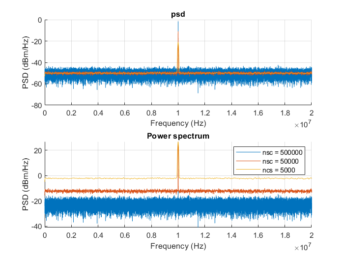
Add a little noise to your pure tone, and notice how the noise power stays the same but signal power fluctuates when you change nsc with the PSD, and how the opposite is true when using the Power Spectrum:

To replicate:

close all
fs = 20e7;
sine = dsp.SineWave('Amplitude',1,'Frequency',10e6,'SampleRate',fs,'SamplesPerFrame',1000000);
y = sine();
y = y+ randn(length(y),1);

figure(1)
subplot 211
title('psd')
hold on
subplot 212
title('Power spectrum')
hold on
for method = {'psd', 'power'}
    for nsc = [500000, 50000, 5000]
        nov = floor(nsc/2);
        nff = max(256,2^nextpow2(nsc));

        [pxx, f] = pwelch(y,rectwin(nsc),nov,nff,fs, string(method));
        pxx = 10*log10(pxx) + 30; % also convert to dBm
        
        if strcmp(string(method), "psd")
            subplot 211
            ylabel("PSD (dBm/Hz)");
        else
            subplot 212
            ylabel("PS (dBm)");
        end
        plot(f, pxx);
        grid on;
        xlim([0 20e6]);
        xlabel("Frequency (Hz)");
        
    end
end
legend('nsc = 500000', 'nsc = 50000', 'nsc = 5000');