Order analysis on sample vibration data to detect unbalance in python

Question

My main goal is to figure out how to do an order analysis in Python. For this I'm trying to do an order analysis in python to some sample vibration data I found here (with and without unbalance).

I got informations on how to do an orderanalysis here and informations on how to resample the data from the time domain to the angle domain here.

The setup:

The setup for the simulation of defined unbalances and the measurement of the resulting vibrations is powered by an electronically commutated DC motor [...], which is controlled by a motor controller [...].

Vibration sensors (PCB Synotech GmbH, type PCB-M607A11 / M001AC) are attached to both the bearing block and the motor mounting and are read out using a 4-channel data acquisition system (PCB Synotech GmbH, type FRE-DT9837).

Using the setup described in above section, vibration data for unbalances of different sizes was recorded. The vibration data was recorded at a sampling rate of 4096 values per second.

In total, datasets for 4 different unbalance strengths were recorded as well as one dataset with the unbalance holder without additional weight (i.e. without unbalance). The rotation speed was varied between approx. 630 and 2330 RPM in the development datasets [...]. Each dataset is provided as a csv-file with five columns:

1. V_in        : The input voltage to the motor controller V_in (in V)
2. Measured_RPM   : The rotation speed of the motor (in RPM; computed from speed measurements using the DT9837)
3. Vibration_1     : The signal from the first vibration sensor
4. Vibration_2     : The signal from the second vibration sensor
5. Vibration_3     : The signal from the third vibration sensor

I used data set 0D.csv (no unbalance) and data set 4D.csv (strong unbalance) to compare the difference.

My try to do an order analysis in python on this data:

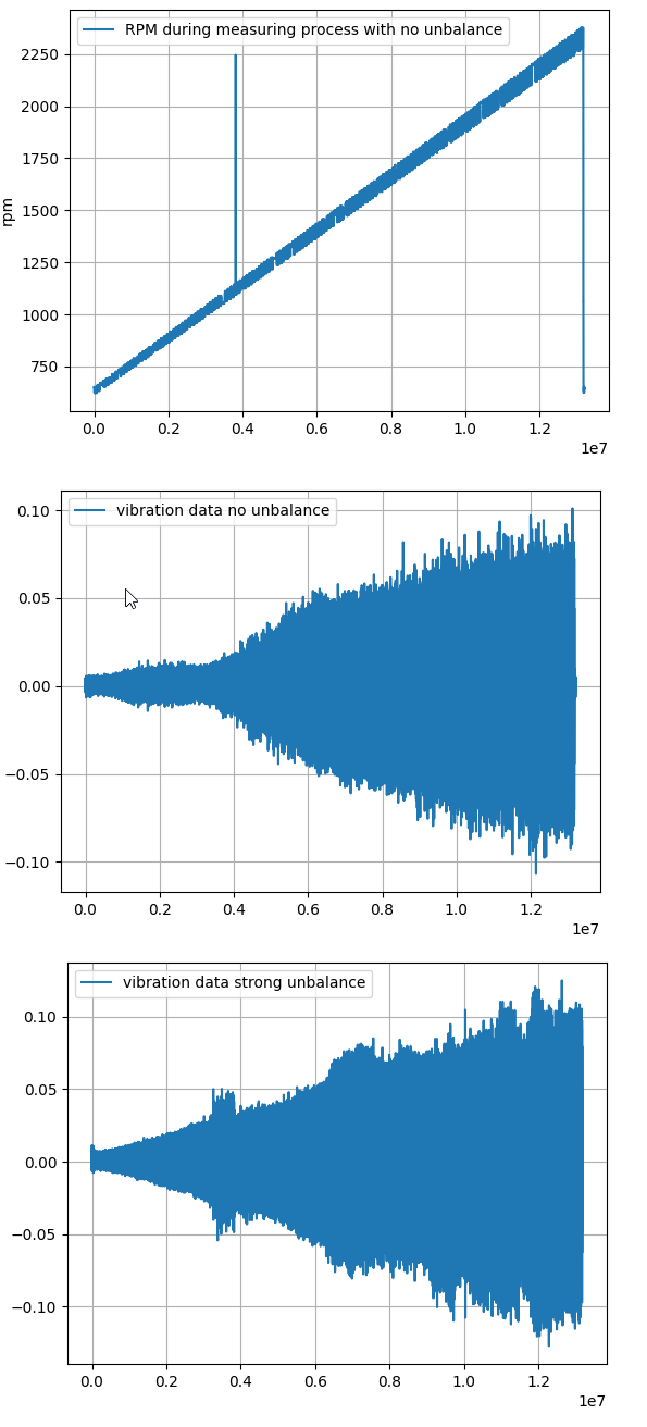
First I loaded the data into a pandas dataframe and then extracted data of both data_sets for "Vibration_1" and "Measured_RPM" and plottet them:

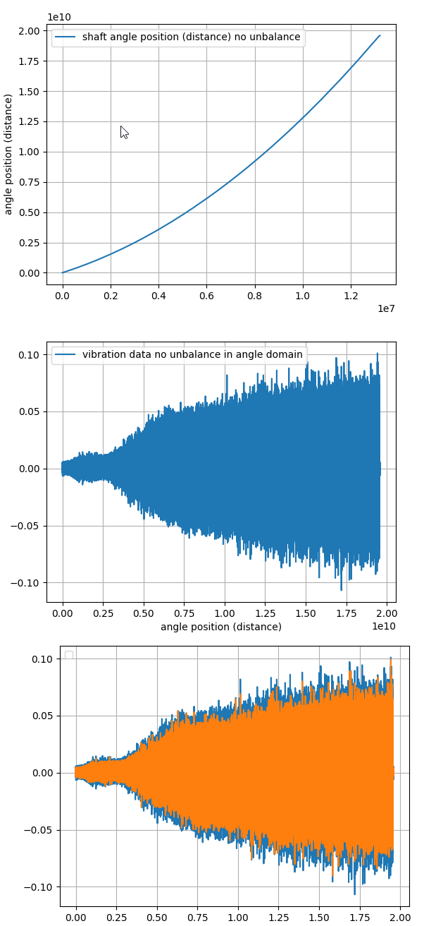
Then I followed some steps here to resample the data from the time domain to the angle domain. First I plottet the angle position, then the vibration data in angle domain. Then I resampled the data. The third picture shows the plots of the "old" vibration signal (blue) and the resampled vibration signal (orange).

# Integrate the speed signal to obtain shaft angle position
distance = np.cumsum(rpm)

# resampling data
x = distance
y = vibration_data
f = interp1d(x, y)
xnew = np.linspace(min(distance), max(distance), num=len(distance))
ynew = f(xnew)

I made an FFT an plottet the result (here I hand the sample rate of 4096 Hz over to the fft but I think that is not correct, I assume I have to hand over samples per revolution but how do I get those?):

# fft with the new sampled data (own function which eleminates DC component, low-passes at sample_rate*0.4 and windowed the signal)
# ynew: resampled vibration data
sample_rate = 4096
fft_freq, fft_amplitude = filter_window_fft(ynew, sample_rate)

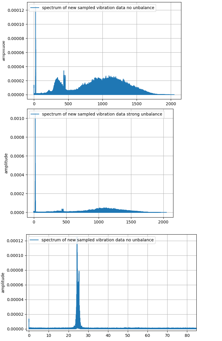
This gives me this spectrums (the third spectrum is the zoomed in variant of no unbalance data):

I would have expected a peak at 1 (1. Order) instead there is a high peak at 25.

Then I had the idea to convert the rpm in rps (rotation per second) and then devided by samples per second to get the rotations, here I am not sure if that is the correct way.

# rpm in rps (rotation per seconnd) and then devided by samples per second to get rotations
rot = (rpm / 60) / sample_rate

# Integrate the rotation signal to obtain shaft angle position
distance = np.cumsum(rot)

# resampling data
x = distance
y = vibration_data
f = interp1d(x, y)
xnew = np.linspace(min(distance), max(distance), num=len(distance))
ynew = f(xnew)

fft_freq, fft_amplitude = filter_window_fft(ynew, sample_rate)

This gives me this spectrums (the second and third plot are zoomed in):

But that doesn't seem to look any better.

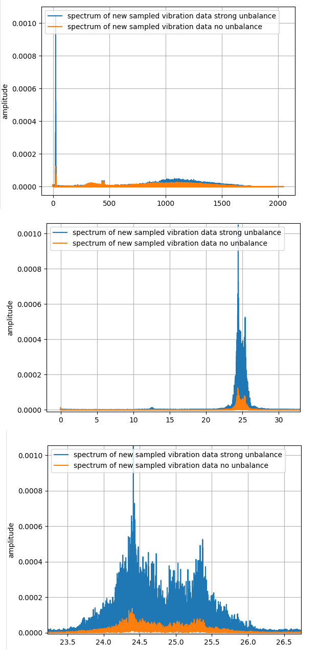
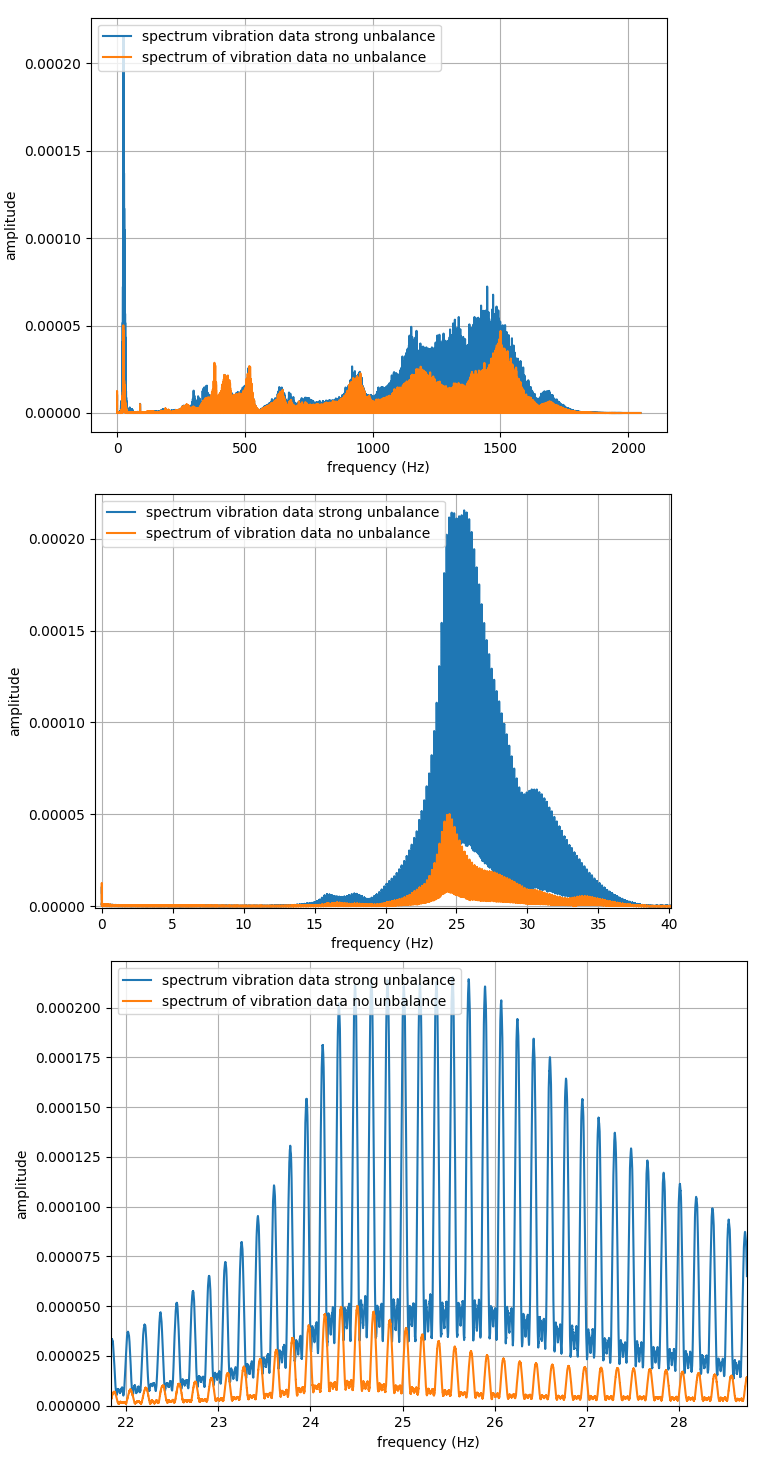
Then just for fun I plottet the fft spectrum of the "normal" vibration data without tranforming them into angle domain. Then I got this plots (second and third plots are zoomed in):

Zooming in let many peaks appear. I'm wondering where do they come from? Do they come from the variable rotation speed?

My Questions:

• Did I get the right plots?
• If not, what am I doing wrong? What is the correct way in doing an order analysis in Python? Or what are the correct steps in doing an order analysis in general?
• What should I hand over as sample rate for the fft? Samples per revolution? How do I get those?
• Where do those peaks in the "normal" spectrum come from?

If any more informations or plots are required I will add them here. Thank you for your time and any help!

Whole Python-Code:

# loading no unbalance data
data_0D_train = pd.read_csv('path/to/csv/0D.csv')
# loading strong unbalance data
data_4D_train = pd.read_csv('path/to/csv/4D.csv')

# reducting data to process faster
rpm = data_0D_train.Measured_RPM[13211647:].to_numpy()
   
# reducting data to process faster
vibration_data = data_0D_train.Vibration_1[13211647:].to_numpy()
    
sample_rate = 4096

# rpm in rps (rotation per seconnd) and then devided by samples per second to get rotations
rot = (rpm / 60) / sample_rate

# Integrate the speed signal to obtain shaft angle position (distance) 
distance = np.cumsum(rot)
   
# resampling data
x = distance
y = vibration_data
f = interp1d(x, y)
xnew = np.linspace(min(distance), max(distance), num=len(distance))
ynew = f(xnew)

# fft
fft_freq, fft_amplitude = filter_window_fft(ynew, sample_rate)

---

Update:

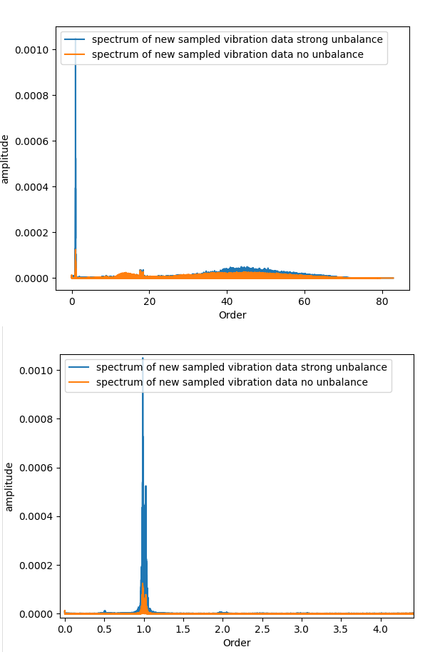
I think I solved the Problem: I forgot to hand over the "new" sample rate to the fft. For this I used the value-distance of the new resampled x-axis and calculated the inverse value to get the new sample rate.

This gives me finally the plot I would have expected:

But I'm still not shure if I'm missing important steps to realize an order analysis.

I would really appreciate a short feedback on this. Thank you!

New Python code:

# round per sample
round_per_sample = (rpm / 60) / sample_rate

vibration_data = data_0D_train.Vibration_1[13211647:].to_numpy()

# itegrate the speed signal to obtain shaft rounds position
shaft_rounds_position = np.cumsum(round_per_sample)

# resample data
x = shaft_rounds_position
y = vibration_data
f = interp1d(x, y)
xnew = np.linspace(min(shaft_rounds_position), max(shaft_rounds_position), num=len(shaft_rounds_position))
ynew = f(xnew)

# new sampele rate out of value-distance of new x-axis
new_periodtime = xnew[2] - xnew[1]
new_sample_rate = 1/new_periodtime

# fft
fft_freq, fft_amplitude = filter_window_fft(ynew, new_sample_rate)

Answer 1

I think you are doing basically right, you can selectively add two more steps:

(1) Check max order for a new sampling rate in order domain, make sure you avoid aliasing.

(2) Add some flexibility to up-sample or decimate data, now your sampling rate in order domain is determined by your sampling rate in time domain.