5
$\begingroup$

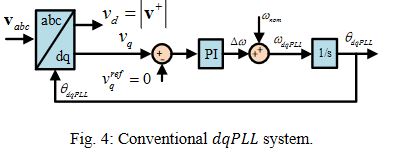
I am going to implement in C++ software the synchronous frame phase locked loop (SFPLL) for estimation of angle and frequency of the three phase grid 220V/50Hz.

enter image description here

For the internal PI controller setting I have decided to use the design by emulation method i.e. design the controller as if the system to be continuous, transform the PI controller into the discrete domain and verify the design in discrete simulation.

  1. PI controller design for continuous system

I have chosen the root locus design method for its clarity. The closed loop transfer function of the SFPLL (in case the grid voltages have amplitudes equal to unity) is

\begin{equation} H(s) = \frac{\left(K_p + \frac{K_i}{s}\right)\cdot\frac{1}{s}}{1 +\left(K_p + \frac{K_i}{s}\right)\cdot\frac{1}{s}} = \frac{K_p\cdot s + K_i}{s^2 + K_p\cdot s + K_i}. \end{equation}

In case I compare the characteristic polynomial with the characteristic polynomial of second order system $s^2 + 2\cdot\zeta\cdot\omega_n\cdot s + \omega_n^2$ I have following formulas for the PI controller parameters

\begin{eqnarray} K_p &=& 2\cdot\zeta\cdot\omega_n \Rightarrow \zeta = \frac{K_p}{2\cdot\omega_n} = \frac{K_p}{2\sqrt{K_i}} = \frac{\sqrt{K_p\cdot T_i}}{2} \\ K_i &=& \omega_n^2 \Rightarrow \omega_n = \sqrt{K_i} = \sqrt{\frac{K_p}{T_i}} \end{eqnarray} i.e. \begin{eqnarray} T_i = \frac{2\cdot\zeta}{\omega_n} \end{eqnarray}

Based on the following formula for the settling time

\begin{eqnarray} t_s = \frac{4.6}{\zeta\cdot\omega_n} = \frac{4.6}{\sigma} \end{eqnarray}

I have final formulas for the PI controller parameters design

\begin{eqnarray} K_p &=& 2\cdot\zeta\cdot\omega_n = 2\cdot\sigma = 2\cdot\frac{4,6}{t_s} = \frac{9,2}{t_s} \\ T_i &=& \frac{2\cdot\zeta}{\omega_n} = \frac{2\cdot\zeta}{\frac{4,6}{\zeta\cdot t_s}} = \frac{\zeta^2\cdot t_s}{2,3} \end{eqnarray}

I have chosen the damping ratio $\zeta=0,7$ and settling time $t_s=0,02\,s$ (one period of the grid 50 Hz). Based on that I have $K_p=460\,\mathrm{Hz/V}, T_i=0,0043\,\mathrm{s}$. In respect to the real value of the amplitude of the grid voltage I have $K_p=\frac{460}{220\cdot\sqrt{2}}\,\mathrm{Hz/V}$.

  1. Transformation of the PI controller into the discrete domain

I have chosen the trapezoidal integration rule for the transformation and I have set the sampling period to the value $50\,\mu s$.

  1. Design verification

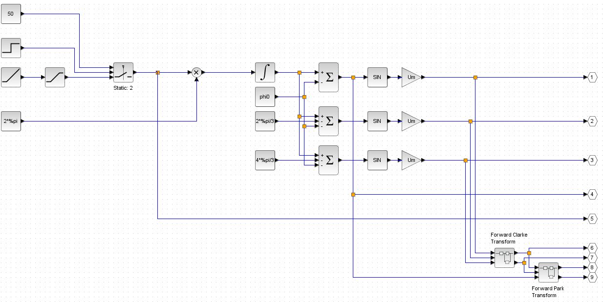
I have developed a simulation of the SFPLL in the Scilab/Xcos software.

enter image description here

a) Grid model

The model simulates three phase grid 220V/50 Hz connected at $t=0.04\,\mathrm{s}$ and with the intial phase $\phi_0=\frac{\pi}{2}$.

enter image description here

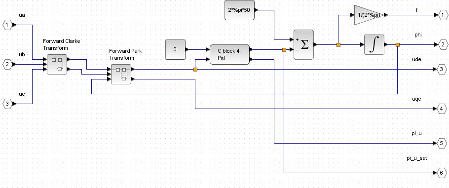
b) SFPLL model

The model of the PLL

enter image description here

The C block contains following C language code

#include "scicos_block4.h"
#include "stdio.h"

#define reference_value          ((double *)GetRealInPortPtrs(block, 1))
#define actual_value             ((double *)GetRealInPortPtrs(block, 2))
#define action_value             ((double *)GetRealOutPortPtrs(block, 1))
#define unsaturated_action_value ((double *)GetRealOutPortPtrs(block, 2))

// parameters
#define Kp (GetRparPtrs(block)[0])
#define Ti (GetRparPtrs(block)[1])
#define T  (GetRparPtrs(block)[2])
#define Min  (GetRparPtrs(block)[3])
#define Max  (GetRparPtrs(block)[4])

typedef struct
{
    double error;
    double proportional_increment;
    double integral_increment;
    double action_increment;
    double tmp;
    double error_previous;
    double action_previous;
}Pid_work;

FILE *dump_file;

void Pid(scicos_block *block,int flag)
{

  Pid_work *work;

  if (flag == 4) 
  {
     /* init */
    if((*(block->work) = (Pid_work*)scicos_malloc(sizeof(Pid_work))) == NULL)
    {
        set_block_error(-16);
        return;
    }
    work = *(block->work);  
    work->error = 0;
    work->proportional_increment = 0;
    work->integral_increment = 0;
    work->action_increment = 0;
    work->tmp = 0;      
    work->error_previous  = 0;
    work->action_previous = 0;

    dump_file = fopen("PI_dump.txt", "w");

    fprintf(dump_file, "Kp, Ki, Action_Min, Action_Max, Action_Saturated, Action_Unsaturated \n");
    fprintf(dump_file, "==================================================================== \n");
  
  } else if(flag == 1) {
   
    work = *(block->work);

    work->error = reference_value[0] - actual_value[0];
    work->proportional_increment = Kp*(work->error - work->error_previous);
    work->integral_increment = Kp*T/(2*Ti)*(work->error + work->error_previous);
    work->action_increment = work->proportional_increment + work->integral_increment;
    work->tmp = work->action_previous + work->action_increment;

    unsaturated_action_value[0] = work->tmp;

    if(work->tmp > Max)
    {
        action_value[0] = Max;
    }
    else if(work->tmp < Min)
    {
        action_value[0] = Min;
    }
    else 
    {
        action_value[0] = work->tmp;
    }

    fprintf(dump_file, "%f, %f, %f, %f, %f, %f \n", Kp, Kp*T/(2*Ti), Min, Max,   action_value[0], work->tmp);

    work->action_previous = action_value[0];
    work->error_previous = work->error;
    
  } else  if (flag == 5) {
    /* ending */
    scicos_free(*(block->work));
        fclose(dump_file);
  }
}

c) Grid voltages reconstructor

This block reconstructs the grid voltages based on the angle, $u_d$ and $u_q$ values computed by the PLL.

enter image description here

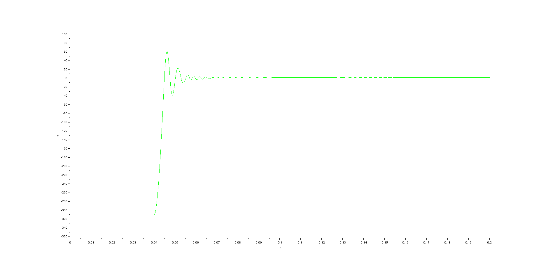
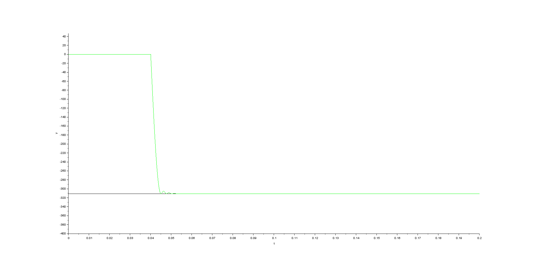
As far as the outcomes of the simulation

  1. $u_d$ vs $u_{d_e}$

enter image description here

  1. $u_q$ vs $u_{q_e}$

enter image description here

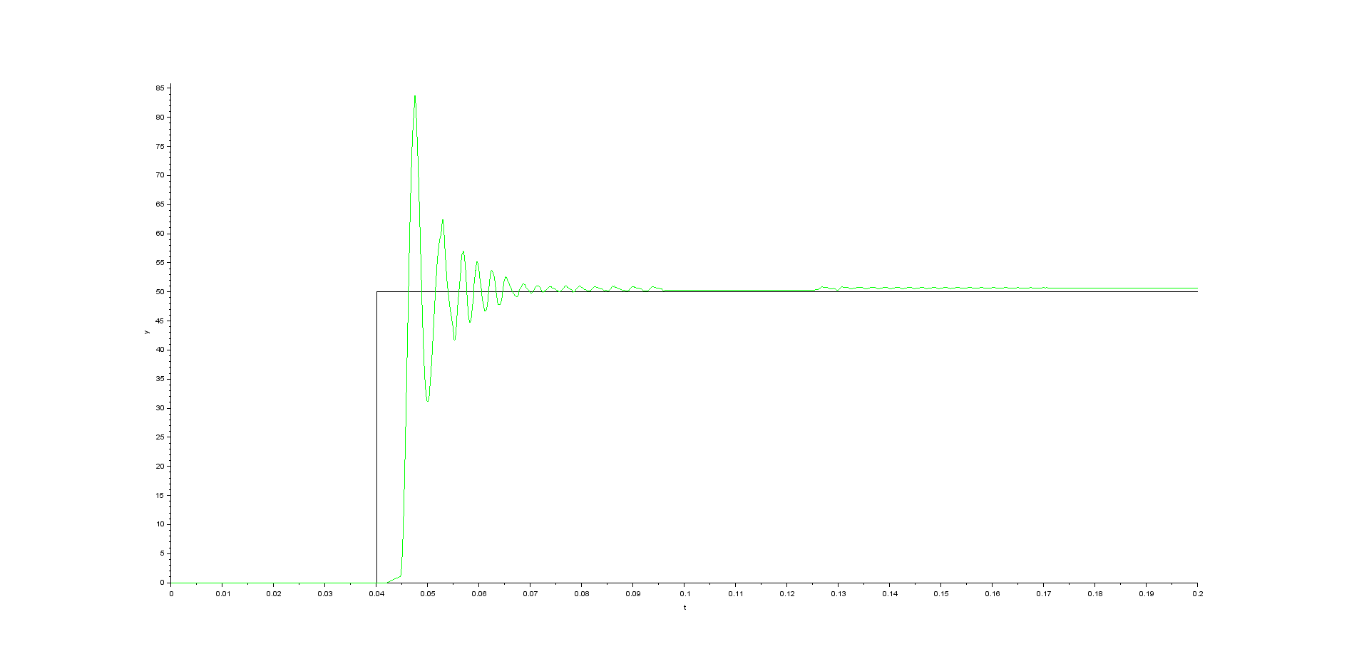
  1. $f$ vs $f_e$

enter image description here

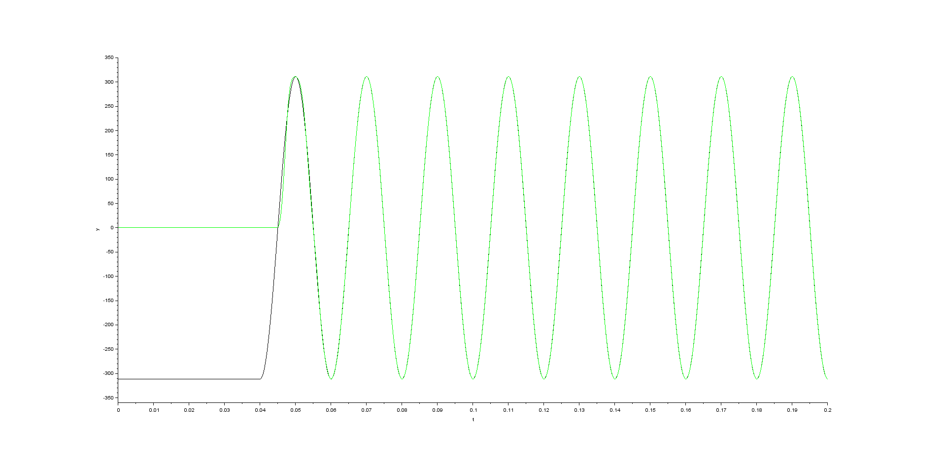
  1. $u_a$ vs $u_{a_e}$

enter image description here

I am surprised by the huge overshoot of the frequency despite the chosen damping ration value 0,7 and small sampling period (it corresponds to 400 samples per one period of the grid). Can anybody tell me what is the reason of the huge frequency overshoot?

$\endgroup$
8
  • $\begingroup$ I didn't have time to read through this all yet Steve but just wanted to check if you properly scaled your integration by T as the sampling interval? When this happens to me it is usually because of this. $\endgroup$ Commented May 31, 2021 at 2:32
  • $\begingroup$ @DanBoschen thank you for your reaction. As far as the integration gain I have been using this $K_i = \frac{K_p\cdot T}{2\cdot T_i}$, where $T$ is the sampling interval. $\endgroup$
    – Steve
    Commented May 31, 2021 at 6:19
  • $\begingroup$ Do I understand correctly or did you mean something else by the integration scaling? $\endgroup$
    – Steve
    Commented May 31, 2021 at 11:08
  • $\begingroup$ What was the constant you came up with for $K_p$ from your continuous time derivation, and then what did you end up using in your discrete time simulation and what is your sampling rate? $\endgroup$ Commented May 31, 2021 at 13:49
  • 1
    $\begingroup$ @Ben Yes, I did. Based on the root locus design $K_p=460\,\mathrm{Hz/V}$ but the actually used $K_p=\frac{460}{\sqrt{2}\cdot 220}=1.478\,\mathrm{Hz/V}$. $\endgroup$
    – Steve
    Commented Jun 1, 2021 at 5:18

2 Answers 2

5
$\begingroup$

Two suggestions to move forward:

  • Reduce $K_i$ to the point of an acceptable overshoot (this will provide the bottom line answer for comparison to the computations.

  • Do system identification (Bode plots) on the open loop system and individual components to isolate the difference between implementation and loop model; the computations were compared below leaving the possibility of a false assumption and this will help isolate that.

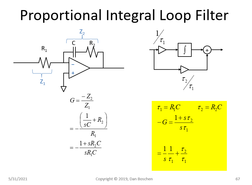
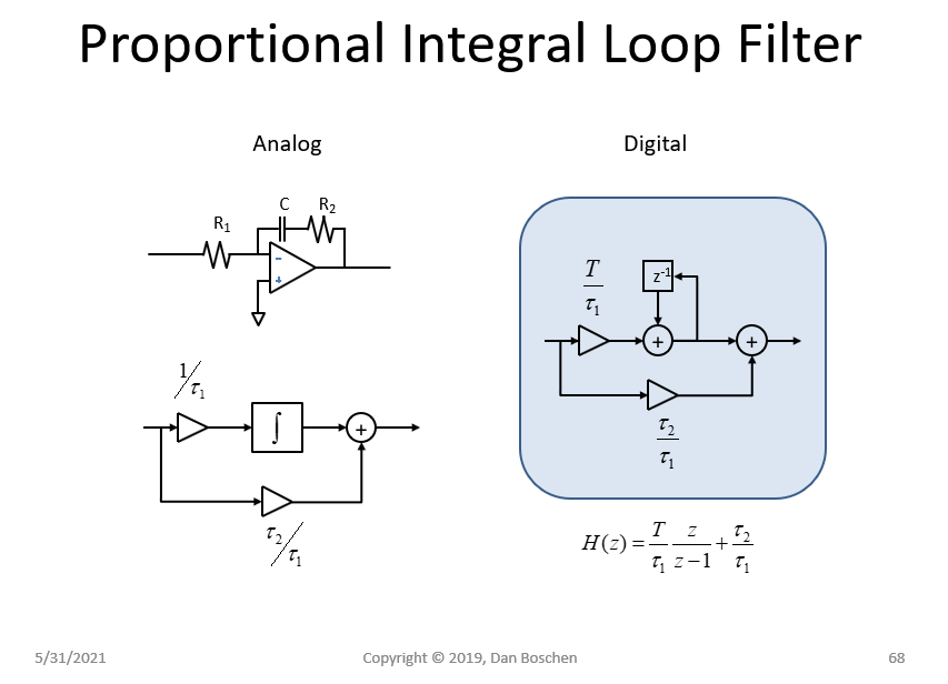
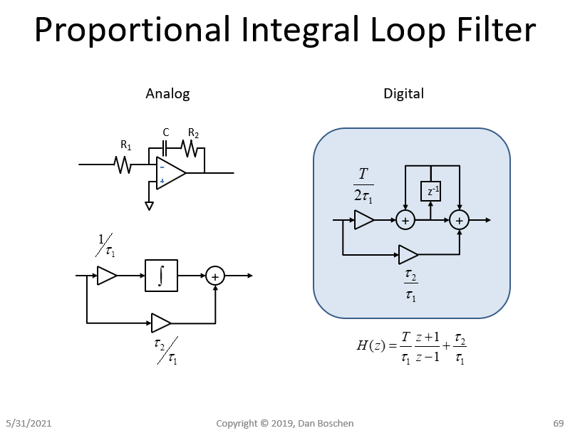
Below shows the similar process in converting from a continuous time to discrete time simulation of a 2nd order PI control loop which after scaling by the amplitude results in similar $K_p$ and $K_i$ values. One possible culprit may be in the actual implementation of the loop filter. Details below for comparison:

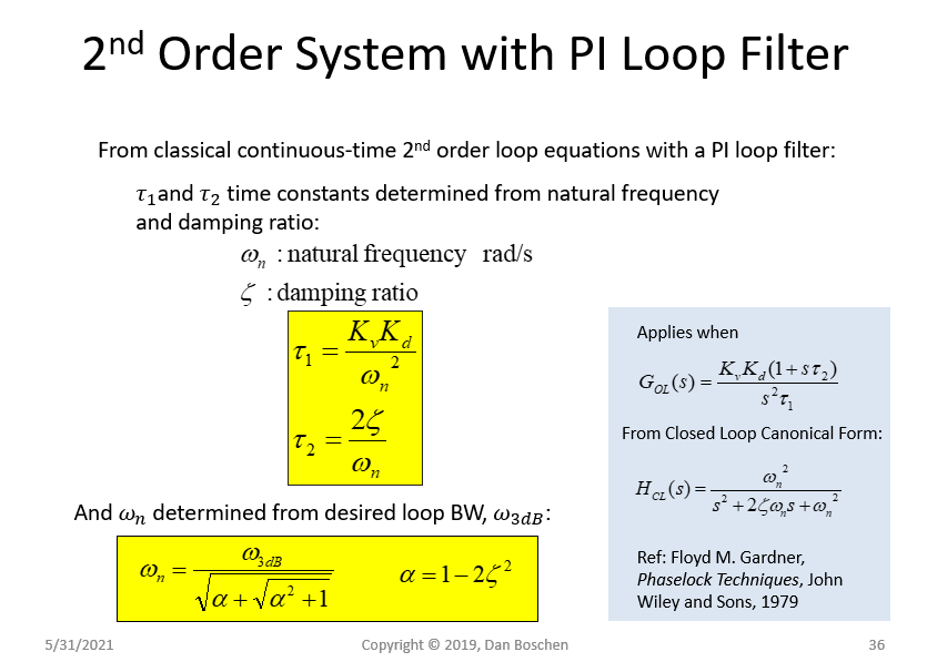
2nd order system

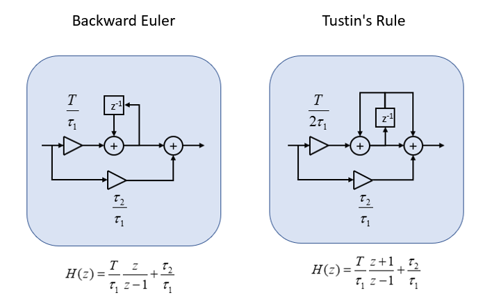
With the loop filter implemented in discrete time as follows:

discrete time loop filters

The equations in continuous time appear to match the OP's derivation from the characteristic equation in the 2nd order canonical form, however it is not clear to me that it was properly implemented to discrete time.

Using a natural frequency $\omega_n = 328.6$ rad/sec (from the OP's settling time) and $K_vK_d = 1$, I get the following for $\tau_2$ and $\tau_1$:

$$\tau_2 = \frac{2\zeta}{\omega_n} = 2(0.7)/(328.6)^2 = 0.0426$$

$$\tau_1 = \frac{K_vK_d}{\omega_n^2} = 1/(328.6)^2 = 9.26e-6$$

Calculating $K_p$:

$$K_p = \frac{\tau_2}{\tau_1} = 0.0426/9.26e-6 = 460$$

$T$ for the OP is 50 us, resulting in $K_i$ as follows:

$$K_i = T/\tau_1 = 50e-6/9.26e-6 = 5.4$$

(or half of the above determined value if the loop filter is indeed implemented per the Tustin's method for the integrator as shown in the block diagram above).

After amplitude scaling by dividing by $\sqrt{2}(220)$ the results for $K_p$ and $K_i$ match what he wrote in the comments below the question (using the Tustin integrator method):

$$K_p = 460/(\sqrt{2}(220)) = 1.478$$

$$K_i = 5.4/(2\sqrt{2}(220)) = 0.00868$$

Below for direct comparison to the OP's implementation are shown the mapping of a continuous time PI Loop Filter to two possible digital implementations (The first uses the method of impulse invariance which for a simple integrator is the backward Euler, and the second uses the Bilinear Transform or Tustin's Rule which is the same as the trapezoidal rule).

PI Loop Filter

Discrete Implementation of PI using Backward Euler Rule:

Impulse Invariance

Discrete Implementation of PI using Trapezoidal Rule (Tustin’s):

Tustins

$\endgroup$
3
$\begingroup$

1 There's a mistake in the PID connection. You must feed the quadrature component, i.e $U_q$ to the PID, not $U_d$. The setpoint of your PLL is $U_q = 0$ because you want your PLL to be in phase with your 3-phase input i.e. $U_d = 1, U_q = 0$.

2 - Perhaps there are hidden delays in the block you instantiated ?

3 - Notice the error equation of your PLL is not linear

$error = sin(\theta_{grid} - \theta_{PLL})$

The equation is approximately linear if $\theta_{grid} \approx \theta_{PLL}$ then $error \approx \theta_{grid} - \theta_{PLL}$

If the initial phase of your PLL is 90 degrees out of phase compared to your input, your theoretical settling time will not be accurate as you are in a non-linear zone of operation. Try your PLL with a 10-degree difference, your settling time should be closer to the theoretical performance.

I noticed that in your first schematic, you use the sine of the phase. You should use the cosine instead. Remember, when the phase of your PLL is 0, the amplitude of $V_a$ should be reach the positive maximum.

4 - I worked with a designer of the 3-phase PLL in the Matlab toolbox, he told me that this DQ-PLL has a metastable state with the PLL being 180 degrees out of phase. The $U_q$ component will be 0 while the $U_d$ component will be -1, instead of +1.

$\endgroup$
6
  • $\begingroup$ If it was 90 degrees out of phase from the ideal discriminator crossing, the loop would just drive it to that ideal lock point- right Ben? $\endgroup$ Commented Jun 2, 2021 at 1:11
  • 1
    $\begingroup$ Yes, but since the equation is non-linear the settling time will be longer than expected $\endgroup$
    – Ben
    Commented Jun 2, 2021 at 11:08
  • $\begingroup$ Right- too bad I'm only allowed one upvote :(. Maybe better to call it acquisition time though as i consider settling time to be that for a step response in the small signal linear region while tracking (acquisition times are typically non-linear and much longer than the settling time in tracking). Minor detail, good answer. $\endgroup$ Commented Jun 2, 2021 at 11:12
  • $\begingroup$ but if you think about it, it is completely arbitrary where the phase is when first starting so the effect really is the final phase between the output and input when locked but shouldn’t even change acquisition time unless we could force that input phase condition - which isn’t realistic, agree?) $\endgroup$ Commented Jun 2, 2021 at 11:23
  • 1
    $\begingroup$ I agree. The initial phase is random. I'm just saying that settling time equations can help select the initial parameters but then one should run simulations to adjust the parameters. $\endgroup$
    – Ben
    Commented Jun 2, 2021 at 11:38

Your Answer

By clicking “Post Your Answer”, you agree to our terms of service and acknowledge you have read our privacy policy.

Not the answer you're looking for? Browse other questions tagged or ask your own question.