All-pass phase compensation only in a specific frequency range

Question

I am trying to design an all-pass filter in order to compensate the phase distortion at the output of an equalizer. To do so, I take the phase vector of the output, compute the real and imaginary part using $e^{j\phi}$, then I do an IFFT and save the time-reversed output. The saved impulse response of the all-pass filter looks like this:

Problems start when I try to restrict the working range of the all-pass equalizer: for example, let's say that the phase compensation needs to work only in 400-16k Hz range, leaving the remaining frequencies uncompensated. To do so, I'm essentially zeroing the phase outside the working range before computing the real and imaginary parts. Probably this is not the correct way, since the resulting impulse response has several ringings at the start and the end of the plot, as you can see from the following picture.

Could you please help me to understand which is the problem here?

EDIT in response to @Dan Boschen's answer

This is the solution I implemented in Octave following your suggestions:

h = read_dat("heqm.dat"); % the IR to equalize
NFFT = length(h);

H = fft(h,NFFT);
ph = unwrap(angle(H));

x = 1:NFFT;
p = polyfit(x,ph,1);
f = polyval(p,x);
f = f-f(1);
figure; plot(ph); hold on; plot(f);

The corresponding plot is:

EDIT 2 The real(ifft(exp(1j*ph))) is:

Next, the definition of the mask:

f1 = 100;
f2 = 300;
half_mask = zeros(1,NFFT/2+1);
half_mask(f1:f2) = 1;
mask = [half_mask, fliplr(half_mask(2:end-1))];
idx = find(mask);

res = f;
res(idx) = ph(idx);
figure; plot(res);

which corresponds to:

Finally, the IR computation:

imp = real(ifft(exp(1j*res)));
figure; plot(imp)

which unfortunately has aliasing:

Did I do something wrong?

Answer 1

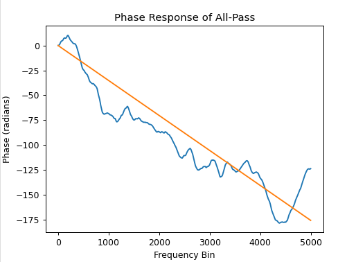
The following demonstrates an approach close to what the OP describes that does not lead to the time domain aliasing experienced. Specifically, the average delay of the filter is determined and for that linear slope of phase versus frequency- all frequencies that are not to be modified by the equalizer are to be replaced with that linear phase slope. (Update: after reviewing OP’s specific waveform the time domain aliasing still exists following this process, and I am concluding that the time span of the equalizer is not supporting the overall time delay given by the waveform - see bottom of post for that detail)

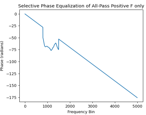
Consider a phase response in the frequency domain as follows from an example 5000 bin DFT, together with a best fin linear line consistent with the average delay of the signal:

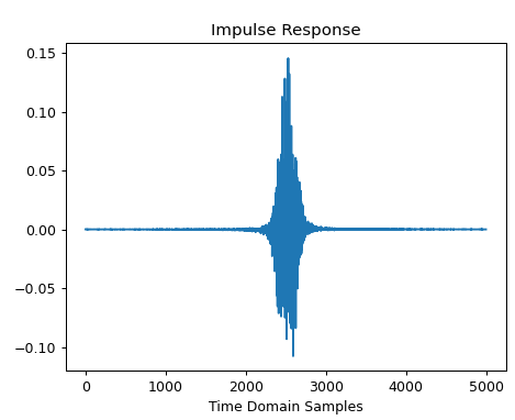
Below is the IFFT prior to any selection

imp = fft.ifft(np.exp(1j*phase))
plt.plot(fft.fftshift(imp))

We note that bin 0 represents "DC", bins 1 through 2500 the positive frequencies, and bins 2501 through 4999 represent the negative frequencies. (With bin 4999 the negative of bin 1, bin 4998 the negative of bin 2, etc).

If we consider this phase response to be the compensation we want, but only isolated to selective frequencies, we have to consider if the signal that we are compensating is real (after compensation, in which case the phase will be conjugate symmetric after compensation) in which case we need to include both positive and negative frequencies, or if the signal is complex and if we only wish to compensate the positive or negative frequency component.

Showing both cases to show that the approach handles both cases without aliasing issues:

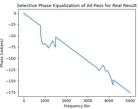
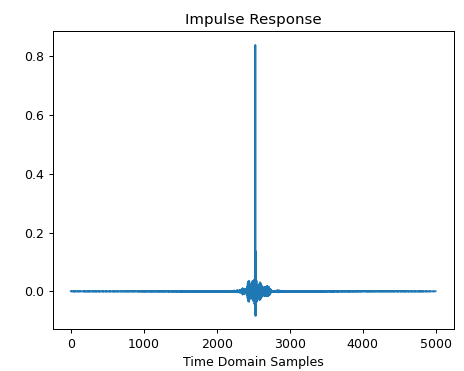
First for a real result after equalization:

f1 = 800
f2 = 1500
N = 5000
mask = np.zeros(N)
mask[f1:f2+1] = 1
mask[N-f1:N+1 -f2] = 1
result = np.where(mask, phase, plin ) 

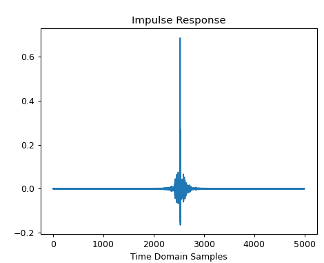
With the following result for the impulse response:

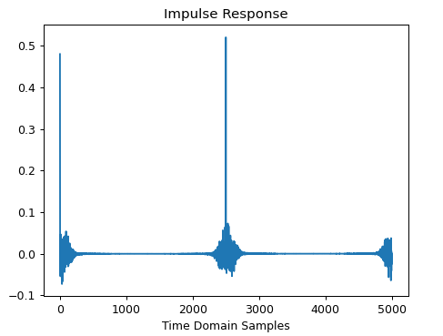
And again for the case of selecting only the positive frequencies:

mask = np.zeros(N)
mask[f1:f2] = 1
result2 = np.where(mask, phase, plin )

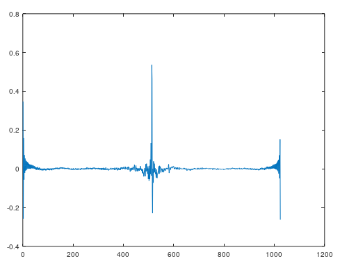
I do not know the specifics of what the OP had done, but the time domain aliasing shown is consistent with zeroing every other bin in the frequency domain. For example for the phase plot shown in the beginning if we zeroed every other sample a similar time domain aliasing would occur:

phase2 = np.copy(phase)
phase2[::2]= 0
imp4 = fft.ifft(np.exp(1j*phase2))
plt.figure()
plt.plot(fft.fftshift(imp4))

UPDATE: I reviewed the OP's data and conclude from that the overall delay is exceeding the time duration of the samples given causing aliasing in the time domain to occur.

Observe the following results:

Out of personal preference, I include fftshift in my plots of the impulse response to center the plot at t=0, plotting positive and negative time as an equivalence to the processing in the frequency domain with positive and negative frequencies. Similar to getting aliasing for frequencies above $f_s/2$ (negative frequencies) we can have similar effects in the time domain for delays above $T/2$ where $T$ is the total time duration of the signal being processed.

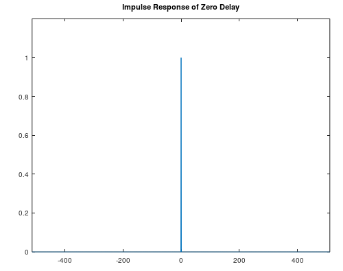
To illustrate, below is the process to plot the impulse response for a vector starting at t=0 with sample 1 followed by 1023 zeros (matching length of the OP's example, and coded on Octave (and instead of taking the real, I plot the complex magnitude):

xaxis = -512:511
plot(xaxis, fftshift(abs(ifft(exp(j*zeros(1024,1))))))):

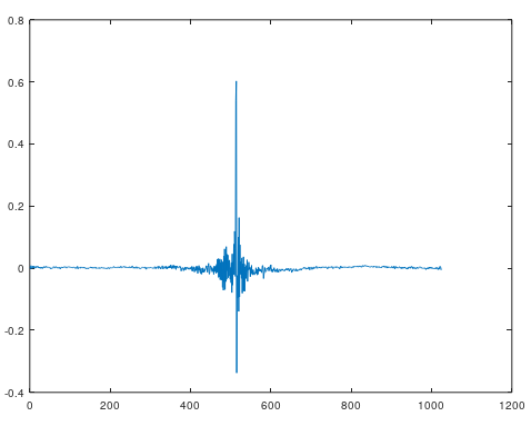
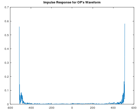
Same processing for impulse response of OP's signal and it is clear that the overall delay has been further shifted beyond half the total time duration which would result in aliasing (consider the impulse response of the equalizer would ideally be centered in the span of the filter while in this case it has gone beyond the filter edge):

plot(xaxis, fftshift(abs(ifft(exp(j*phi)))))):

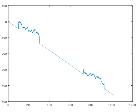
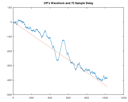
In general, for every delay of one sample, the phase will vary linearly from 0 to $-2\pi$ from DC to the sampling rate. The OP's phase is varying approximately -450 radians over 1024 frequency bins. $450/(2\pi)$ corresponds to a delay of 72 samples

plot(xaxis, fftshift(abs(ifft(exp(j*zeros(1024,1))))))):

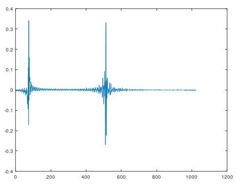
Here is the OP's original waveform along with a 72 sample delay (which would then wrap cleanly at the positive/negative frequency boundary as well, but still resulted in the time domain aliasing the OP has computed):

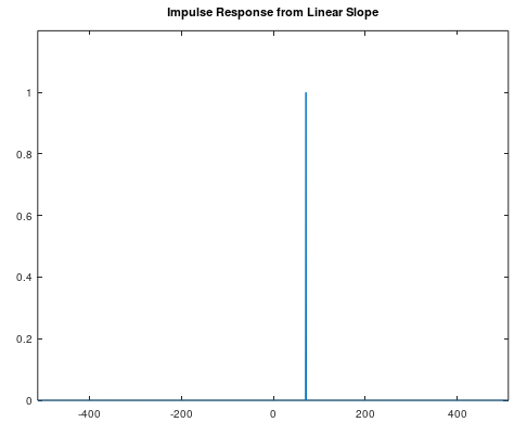
Here is the impulse response computed from the phase of the 72 sample delay to confirm the prior processing:

plot(xaxis, fftshift(abs(ifft(exp(j*f)))))

Conclusion: I am rather surprised that the waveform would have that much additional delay due to the variation of the phase from the best linear fit (as an analogy to frequency translation occurring (in the frequency domain) from phase rotation in time, here we clearly see evidence of time translation (in the time domain) from the same phase rotation process apparently occurring in the frequency domain. Given this, the impulse response is being translated further than the original time sample can support, and the solution would therefore require a longer time sample which should then eliminate the aliasing. (Sometimes it is easier to reverse time and frequency to understand what may be occurring; as it may be more intuitive for many to understand how this could occur with frequency domain aliasing from undersampling--- here it is the same thing except instead of increasing the sampling rate we need to increase the time duration).