How to approximate the transfer function of compensator using root locus?

Question

I have the root locus of a system with and without compensator. The system is consist of a PD-controller and the process, the output is fed back to the controller via $G_s(s) = 1$. The upper graph is the root locus without compensator.
The compensator is in series with the PD-controller.

$$G_1(s) = \frac{G_r(s)G_p(s)}{1+G_r(s)G_p(s)}$$ $$G_2(s) = \frac{G_c(s)G_r(s)G_p(s)}{1+G_r(s)G_p(s)G_c(s)}$$

Here $G_r(s)$ is the transfer function of the controller, $G_c(s)$ the transfer function of the compensator and $G_p(s)$ the transfer function of the process. The system is LTI.

This is how I did it:

The second graph has two new zeros and one extra pole while contains all the zeros and poles of the first graph( system with no compensator), so the compensator looks like: $$G_c(s) =K \frac{(s-z_1)(s-z_2)}{s-p_1}$$ But what about the constant $K$ ? I don't know how to specify it.

Answer 1

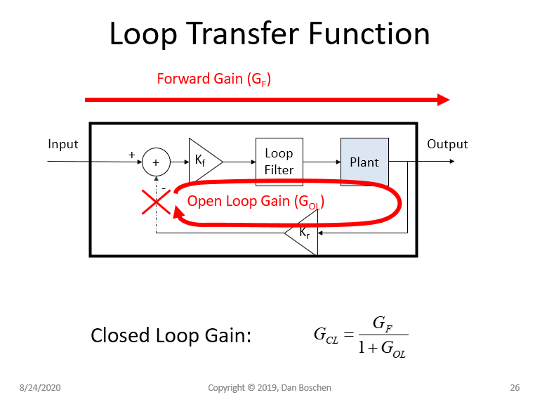
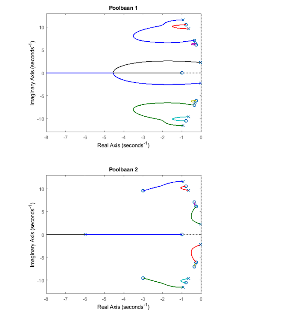
K is the gain parameter for which you will be at any particular point on the root locus. As you increase K, the closed loop poles will start from the open loop poles and move toward the open-loop zeros as depicted in the root locus showing all possible locations of closed loop poles versus gain K.

This is because the general form for the closed loop and open loop gain in a general loop equation is related as:

$$G_{CL}(s) = \frac{G_F(s)}{1+K G_{OL}(s)}$$

Where $G_{CL}(s)$ is the closed loop gain, $G_{F}(s)$ is the forward gain from input to output and $G_{OL}(s)$ is the open loop gain with the real gain $K$ pulled out as a independent variable that we will sweep when creating the root locus plot.

The denominator of the closed loop gain is called the "characteristic equation" and given properness of realizable causal systems (properness means the number of zeros is always less than or equal to the number of poles, not including poles and zeros at infinity), we can determine all loop characteristics (stability, dynamics, etc) from the characteristic equation alone. To really see what is occurring in the root locus plot, consider this equation expressed in terms of poles and zeros of the open loop gain $G_{OL}(s)$ as follows:

$$1+KG_{OL}(s) = 1 + K \frac{G_z(s)}{G_p(s)}$$

Where $G_z(s) = (s-z_1)(s-z_2)...$ is the polynomial of open loop zeros, and $G_p(s) = (s-p_1)(s-p_2)...$ is the polynomial of open loop poles. This is rearranged to be:

$$= \frac{G_p(s)+KG_z(s)}{G_p(s)}$$

Since this equation is in the denominator of the closed loop gain $G_{CL}(s)$ then the roots of the numerator (the zeros of this equation) will be the poles in the closed loop gain!

Knowing that, consider when $K$ is varied from very large to very small: When $K$ is very small then $G_p(s)$ dominates the equation $G_p(s)+KG_z(s)$ and therefore dominates the poles of the closed loop gain. Specifically in this case of very small $K$, the poles of the open loop gain will be the poles of the closed loop gain. Similarly, when $K$ is very large then $G_z(s)$ dominates the equation $G_p(s)+KG_z(s)$ and therefore dominates the poles of the closed loop gain. Specifically in this case of very large $K$, the zeros of the open loop gain will be the poles of the closed loop gain.

This is why the poles start at the open loop poles and move toward the open-loop zeros in the root locus.