Help find the bug in my SPLL code

Question

In an attempt to get myself up to speed with PLLs I'm trying to implement Example 1 from this tutorial, in Python: https://wirelesspi.com/phase-locked-loop-pll-in-a-software-defined-radio-sdr/ (search for "Example 1")

I have output that is close to what the article shows, except that my cos_out[n] seems to be "leaning" to the left:

My phase-difference signale_D[n] is flipped vertically from what the tutorial shows:

I must be missing a - sign or have a sin() where I need cos() but I've checked and triple checked my code.

My code:

import numpy as np
k = 1
N = 15
K_p = 0.2667
K_i = 0.0178
K_0 = 1

samples = np.linspace(0, 100, 100, endpoint=False)
input_signal = np.cos(2*np.pi*(k/N)*samples + np.pi)

integrator_out = 0
phase_estimate = []
e_D = [] #phase-error output
e_F = [] #loop filter output
sin_out = []
cos_out = []

for n, sample_in in enumerate(input_signal):

    # phase detector
    try:
        e_D.append(sample_in * sin_out[n-1])
    except IndexError:
        e_D.append(0)


    #loop filter
    integrator_out += K_i * e_D[n]
    e_F.append(K_p * e_D[n] + integrator_out)


    #NCO
    try: 
        phase_estimate.append(phase_estimate[n-1] + K_0 * e_F[n])
    except IndexError:
        phase_estimate.append(K_0 * e_F[n])

    sin_out.append(-np.sin(2*np.pi*(k/N)*n + phase_estimate[n]))
    cos_out.append(np.cos(2*np.pi*(k/N)*n + phase_estimate[n]))

Answer 1

It is easy to overlook which sample is 'traveling' through the PLL in a for loop at a particular time. Have a look at the PLL block diagram and you will notice that the NCO output is the phase estimate delayed by one sample. Remember that the integrator in the PLL and the integrator in the NCO approximate the integration operation through different rules. There are 3 different methods to implement the integration operation: (a) backward difference, (b) forward difference, and (c) trapezoidal rule. Each of them impacts the pole-zero plot of the system in a different manner.

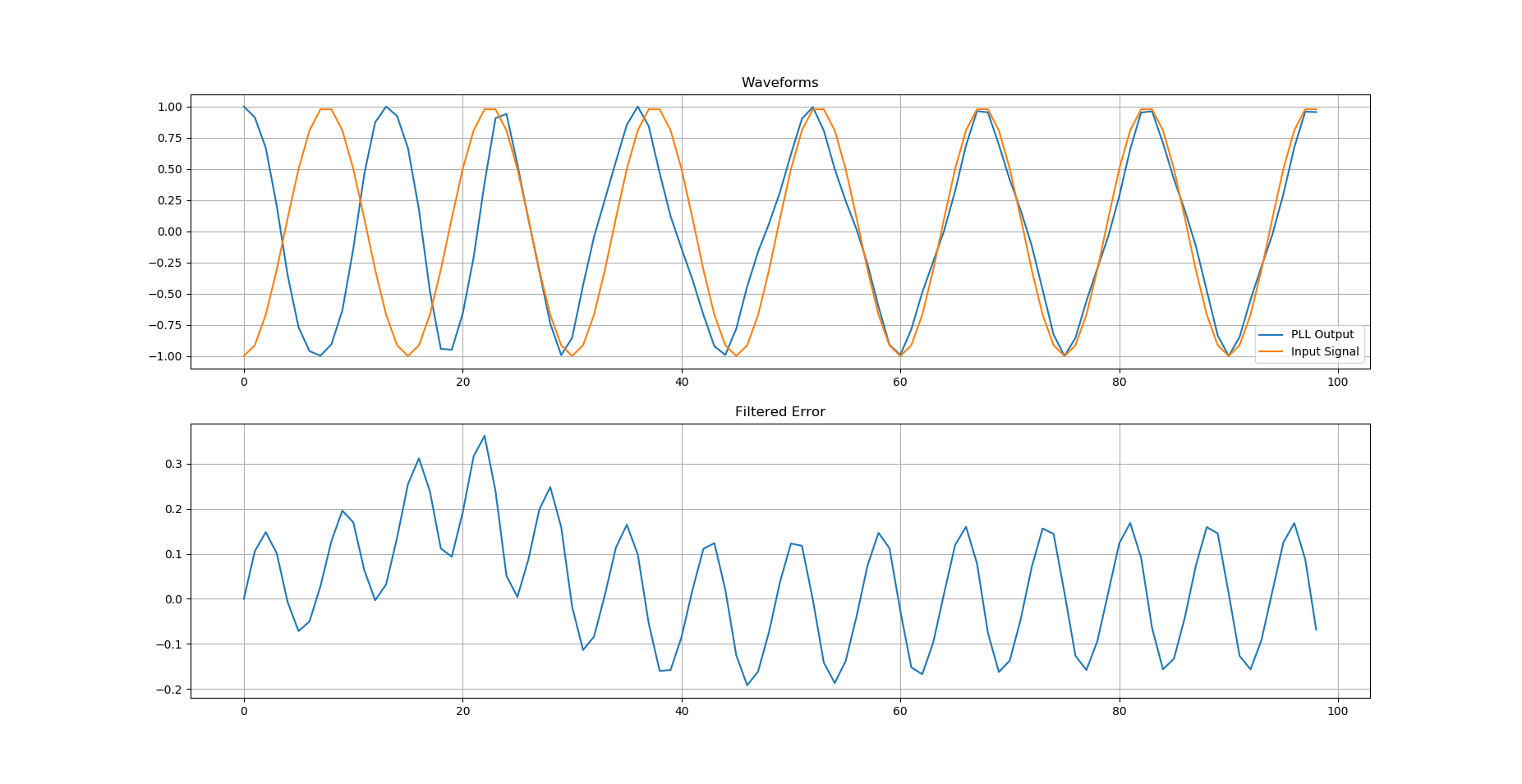
The outputs are plotted below. Your code implemented a different PLL and hence the cosine was leading.

How do we know that this output is correct? Because the lead lag behavior of the PLL output follows exactly that of the filtered error. In the modified code, have a look at how the phase estimate is updated as compared to how it is used in the PLL output signals.

# PLL in an SDR

# Import the necessary packages and modules
import matplotlib.pyplot as plt
import numpy as np

k = 1
N = 15
K_p = 0.2667
K_i = 0.0178
K_0 = 1

input_signal = np.zeros(100)

integrator_out = 0
phase_estimate = np.zeros(100)
e_D = [] #phase-error output
e_F = [] #loop filter output
sin_out = np.zeros(100)
cos_out = np.ones(100)

for n in range(99):
    input_signal[n] = np.cos(2*np.pi*(k/N)*n + np.pi)

    # phase detector
    try:
        e_D.append(input_signal[n] * sin_out[n])
    except IndexError:
        e_D.append(0)


    #loop filter
    integrator_out += K_i * e_D[n]
    e_F.append(K_p * e_D[n] + integrator_out)


    #NCO
    try: 
        phase_estimate[n+1] = phase_estimate[n] + K_0 * e_F[n]
    except IndexError:
        phase_estimate[n+1] = K_0 * e_F[n]

    sin_out[n+1] = -np.sin(2*np.pi*(k/N)*(n+1) + phase_estimate[n])
    cos_out[n+1] = np.cos(2*np.pi*(k/N)*(n+1) + phase_estimate[n])



# Create a Figure
fig = plt.figure()

# Set up Axes
ax1 = fig.add_subplot(211)
ax1.plot(cos_out, label='PLL Output')
plt.grid()
ax1.plot(input_signal, label='Input Signal')
plt.legend()
ax1.set_title('Waveforms')

# Show the plot
#plt.show()

ax2 = fig.add_subplot(212)
ax2.plot(e_F)
plt.grid()
ax2.set_title('Filtered Error')
plt.show()

Answer 2

I've written articles like that, and it's incredibly hard -- and sometimes not the best exposition -- to get the graphs to match exactly with the text. From the looks of things, the author was intentionally showing you idealized graphics rather than the actual output of code.

My phase-difference signale_D[n] is flipped vertically from what the tutorial shows...

Eh, don't worry. It's a control loop, there's always a stray minus sign in there someplace. As long as you match it up with another stray minus sign so that it's stable, you're OK.

I have output that is close to what the article shows, except that my cos_out[n] seems to be "leaning" to the left: cos_out

That's because your K_p is so high. You can get a simple loop, fast settling, or a nice sinusoidal response -- not all three. If you're using the author's numbers, or if you've selected gains to make your loop settle as fast as his idealized example (which was probably chosen more to make things fit in the page rather than because it's the best tuning) then what's happening is that strong signal at the sum frequency is bleeding into the NCO phase, and making the "lean".

Typically a PLL will be set up to take hundreds or thousands of cycles to settle, which implies a much smaller K_p (certainly less than 0.01, and almost arbitrarily small depending on what you're doing). How fast a PLL settles depends on what you're doing, and what you're doing it with, so if your next question is "how fast should it settle" -- I can't answer. But I would say try it for settling in around 100 cycles, 1000, and 10,000. Keep in mind that the capture range (the frequency error between signal and NCO initial frequency over which it can actually acquire a lock) and its tracking performance (its ability to follow a varying input frequency) both go down with slower settling.