The good thing about filters is that they are linear. Therefore you do not need to specify the signal when you are analyzing the filter. You just analyze its impulse response (i.e., filtering an ideal Dirac pulse) and the Fourier transform of that (the transfer function). Based on this analysis, you can judge what the filter would do to any given signal.
For windowing, almost the same is true, just a little backwards: windowing means multiplication in time domain, which is convolution in frequency domain. So it's almost the same as filtering, just exchanging the role of time and frequency domain. Therefore, we can do the same: analyze the window function and its Fourier transform itself, not assuming any specific signal. That's what would happen for a single Dirac pulse in frequency (i.e., a constant DC signal). Then, if you want to know what happens when you window a given signal, just apply convolution in frequency domain (e.g., for a pure tone, that's just shifting it).
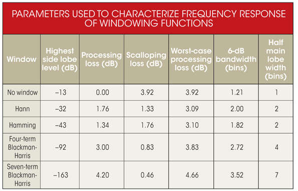
That said, most of the table can be filled by computing the Fourier transform of the window function and then taking the corresponding measurements: how large/wide are the mainlobes, etc. If you cannot compute the Fourier transform analytically, you can try to approximate it, using a Discrete Fourier transform. In this case, use a large $N$, to make sure your estimation errors remain negligible.
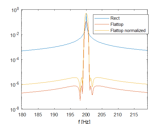
*edit: Regarding your question on the estimation of power: if you want peak heights to be consistent you'll have to normalize your windows accordingly. Since the spectrum of a windowed signal is $X_h(f) = X(f) * H(f)$, i.e., convolution with the spectrum of the window function, the normalization of $H(f)$ matters. For instance, for a small peak to come out in the correct height, you might want to have $H(0)=0$, which means that the coefficients in time domain should sum to one. Alternatively, if you want your windowed signal to behave like the unwindowed one, take into account that applying "no window" means implicitly applying a rectangular window of amplitude 1, so that its coefficients sum to $N$.
In Matlab:
clear;
N = 999;
fs = 2000;
f0 = 200;

taxis = (0:N-1)/fs;
faxis = (0:N-1)/N*fs;
sig = sin(2*pi*taxis*f0);

win = flattopwin(N).';
sig_win = sig.*win;

win_normalized = win/sum(win)*N;
sig_win_normalized = sig.*win_normalized;

figure(1);
clf;
plot(faxis,abs(fft(sig))/N);
hold on;
plot(faxis,abs(fft(sig_win))/N);
plot(faxis,abs(fft(sig_win_normalized))/N);
legend('Rect','Flattop','Flattop normalized')
xlabel('f [Hz]');

set(gca,'YScale','log');
Result (zoomed in around 200):

You can see how with the normalization you can make the flattop window behave like the rectangular window.
Btw: the units of this are not dBm. It's a discrete Fourier transform, transforming Volts into Volts (or unitless quantities into unitless). If you want dBm you have to properly normalize to make sure your FFT approximates a Fourier transform (it involves the sampling time $t_0$) and you'll have to estimate power instead of amplitude.


