This answer discusses the harmonic spectra of the quantized sequence in five cases:
- limit $f/f_s \to 0$,
- synchronous sampling of a cosine with rational $f/f_s$,
- synchronous sampling of a sinusoid of arbitrary phase with rational $f/f_s$,
- asynchronous sampling of a sinusoid with rational $f/f_s$, and
- asynchronous sampling of a sinusoid with rational $f/f_s$ in the limit $L/A \to
0$,
where $f$ is the frequency of the sinusoid, $f_s$ is the sampling frequency, $L$ is the fundamental period of the quantized sequence, and $A$ is the amplitude of the sinusoid. Decibels full-scale (dBFS) shall be referenced to the sinusoid amplitude $A$ at 0 dBFS.
Limit $f/f_s \to 0$
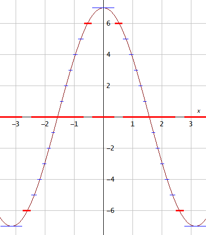
Let the zero-to-peak amplitude of the continuous-time prototypical sinusoid, which is being sampled and quantized, be a positive real number $A$. In the limit $f/f_s \to 0,$ where $f$ is the sinusoid frequency and $f_s$ is the sampling frequency, the amplitudes of the harmonics are found in the Fourier series representation of the continuous-time piece-wise constant quantized waveform. The terms of the Fourier series are directly the harmonics of the fundamental frequency. We can construct the waveform as a sum of components like the red curve here, illustrated for sinusoid amplitude $A = 7$:

Figure 1. prototypical sinusoid, of amplitude $A=7$, and its quantization in blue, with a component highlighted in red.
We are working with cosine instead of a sine because the math is nicer this way. Because of the symmetries, each component has only odd harmonics and only cosine terms in its Fourier series. The non-zero coefficients of the Fourier series of a component of integer amplitude $k \in 1\ldots \operatorname{round}(A)$ are given by:
$$a_n = \frac{4}{\pi}\int_{x_0}^{x_1}\cos(nx)\,k\,dx = \frac{4k}{\pi n}\big(\sin(x_1n) - \sin(x_0n)\big),\quad n\text{ odd},\tag{1}$$
with the component having the said amplitude over the interval $x_0 < x < x_1$ in the first quarter-period of the cosine. I did not bother to explicitly write the contributions from the symmetrically arranged non-zero pieces of the component in the other quarters, because they will contribute identically to the odd harmonic cosine terms in the Fourier series. Instead I simply included the implicit factor 4 in the equation.
The Fourier series of the full piece-wise constant waveform is a sum of the Fourier series of the components. The boundaries of the pieces that we need to include in the sum are:
$$\begin{gather}0 < x < \operatorname{acos}\left(\frac{\operatorname{round}(A) - 0.5}{A}\right),\quad \text{if }k = \operatorname{round}(A),\\
\operatorname{acos}\left(\frac{k + 0.5}{A}\right) < x < \operatorname{acos}\left(\frac{k - 0.5}{A}\right),\quad \text{if }k \in 1\ldots \operatorname{round}(A)-1,\end{gather}\tag{2}$$
where $\operatorname{acos}\left(\frac{s}{A}\right)$ comes from solving $A\cos(x) = s$ in the first quarter-period. The non-zero coefficients of the Fourier series of the full piece-wise constant waveform are then given by:
$$\begin{gather}a_n = \frac{4\operatorname{round}(A)}{\pi n}\,\sin\bigg(\operatorname{acos}\left(\tfrac{\operatorname{round}(A) - 0.5}{A}\right)n\bigg) +\\\frac{4}{\pi n}\sum_{k=1}^{\operatorname{round}(A)-1} \Bigg(k\sin\bigg(\operatorname{acos}\left(\tfrac{k - 0.5}{A}\right)n\bigg) - k\sin\bigg(\operatorname{acos}\left(\tfrac{k + 0.5}{A}\right)n\bigg)\Bigg),\quad n\text{ odd}.\end{gather}\tag{3}$$
The rounding convention does not matter as long as it is to a nearest integer.
8-bit quantization
It is not out of reach to compute Eq. 3 for $A=2^{23} - 1$ and $n \in {5, 7},$ as parameterized in the question, using something like Python's mpmath. Let's try that but with a 8-bit sinusoid first, because we can then evaluate $a_n$ at multiple $n$ in a reasonable time and perhaps learn something from the results. In Python:
import numpy as np
import mpmath as mp
def a_n(A, n):
    if int(n) & 1:
        return 4*mp.floor(A + 0.5)/(mp.pi*n)*mp.sin(mp.acos((mp.floor(A + 0.5)-0.5)/A)*n) + 4/(mp.pi*n)*mp.nsum(lambda k: k*( mp.sin(mp.acos((k-0.5)/A)*n) - mp.sin(mp.acos((k+0.5)/A)*n) ), [1, mp.floor(A + 0.5)-1])
    else:
        return 0

A = 2**7-1  # amplitude (positive real)

for n in np.arange(1, 10**4, 2):
    print(str(n)+","+str(20*mp.log10(mp.fabs(a_n(A, n))/A)))  # n, a_n (dBFS)

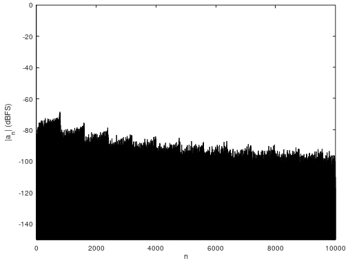
Figure 2. Amplitudes of harmonics of the quantized prototypical sinusoid of amplitude $A=2^{7}-1$. Only odd harmonics are present.
It took some minutes on my PC to get the results (Fig. 2). The graph looks jagged. I think this is because the waveform is similar to a sawtooth riding on a sinusoid, and near the zero crossing the sawtooth frequency stays approximately the same over a large portion of the waveform, being $2\pi A \approx$ 797.964534 times the fundamental frequency at the zero crossing as an asymptotic approximation in the limit $A\to\infty$ of the frequency $\pi/\operatorname{asin}\big((k + 0.5)/A\big)$ calculated based on the distance between the discontinuities of the saw wave just around the zero crossing. Indeed, the largest amplitude is found nearby at $|a_{787}| =$ -68.30 dBFS. This is much higher than the amplitude of a "random" early harmonic. Such peaks are repeated later at approximate harmonics of the sawtooth frequency but less clearly and with a roll off arising from the factor $1/n$ in Eq. 3, making the asymptotic decay -20 dB/decade (~-6 dB/octave) as $n\to\infty$. The amplitude of the fundamental frequency is 0.00066 dBFS, I think because the rounding at the top of the sinusoid is "pulling it up" from the 0 dBFS amplitude of the prototypical cosine.
24-bit quantization
The following continuation of the earlier Python script computes in high precision your desired numbers for $A=2^{23} - 1$, in the limiting case $f/f_s \to 0$:
A = 2**23-1 # amplitude (positive real)

n = 5  # number of the harmonic (odd positive integer)
mp.mp.prec = 70  # Precision 1
20*mp.log10(mp.fabs(a_n(A, n))/A) # in dBFS
mp.mp.prec = 140  # Precision 2
20*mp.log10(mp.fabs(a_n(A, n))/A) # in dBFS

n = 7  # number of the harmonic (odd positive integer)
mp.mp.prec = 70  # Precision 1
20*mp.log10(mp.fabs(a_n(A, n))/A) # in dB
mp.mp.prec = 140  # Precision 2
20*mp.log10(mp.fabs(a_n(A, n))/A) # in dB

mp.mp.prec = 53  # Restore default precision
I'm only reporting as many digits as are agreed about by repeated computation using two different mpmath precision settings, including also the digits that got changed by $\pm1$ due to larger changes in later digits. After a total of a few hours of computation on my PC, the result is that with $A=2^{23} - 1$ and $f/f_s \to 0,$ the amplitude of the 5th harmonic is -226.91150085 dBFS and the amplitude of the 7th harmonic is -226.9115030 dBFS. I also computed the amplitude of the fundamental frequency, 3.9195785E-11 dBFS. I also computed in a full day the amplitudes of a number of higher harmonics, in Python:
A = 2**23-1 # amplitude (positive real)

for m in range(1, 20):
  n = mp.mpf(10)**m+1 # number of the harmonic
  mp.mp.prec = 70  # precision
  a_n_low_prec = a_n(A, n)
  mp.mp.prec = 90  # precision
  a_n_high_prec = a_n(A, n)
  print(str(n)+","+str(20*mp.log10(mp.fabs(a_n_low_prec)/A))+","+str(20*mp.log10(mp.fabs(a_n_high_prec)/A)))  # n, a_n

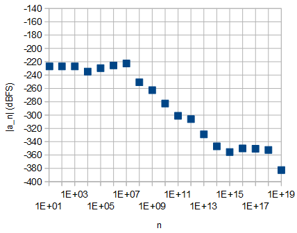
Figure 3. Amplitudes of a selection of odd harmonics of the quantized prototypical sinusoid, with $A=2^{23}-1$.
The corner frequency before the roll-off is again approximately the sawtooth frequency at the zero crossing of the quantized prototypical sinusoid, $2\pi A = 2\pi(2^{23}-1) \approx$ 5.270717225E7 times the fundamental frequency $f$.
Synchronous sampling of a cosine with rational $f/f_s$
Let the prototypical sinusoid, which is being sampled and quantized, be a cosine without a phase shift. That is to say, one of the samples is at the peak of the sinusoid. Let $f/f_s$ be equal to a rational number $c/d$, with $c$ and $d$ integer. The fundamental period $L$ of the periodic sequence of quantized samples is:
$$L = \frac{d}{\operatorname{gcd}(c, d)},\tag{4}$$
where gcd denotes the greatest common divisor. A real discrete Fourier transform (real DFT) of length $L$ has bin frequencies that are the harmonic frequencies of the period-$L$ frequency. The period-$L$ frequency is equivalent to the frequency of the prototypical sinusoid only if the numerator of the irreducible fraction representation of $f/f_s$ equals 1. Otherwise the real DFT bin frequencies contain also other frequencies than those equivalent to in-band harmonics of the sinusoid.
What we have learned from the results so far is that the amplitudes of the harmonics of the quantized prototypical sinusoid do not start to roll off until after the approximately $2\pi A$th harmonic. This means that with rational $f/f_s$, the amplitude of an in-band harmonic frequency of the quantized sequence is typically almost fully determined by aliased frequencies. As an example of such aliasing, with $f_s =$ 48 kHz and $f =$ 1000 Hz, the 5th harmonic gets summed with the aliases of the 43th, 53th, 91th, 101th, 139th, 149th, etc. harmonic:
$$\begin{eqnarray}
&& \ldots\\
&=& 48000\text{ Hz}\times -3 + 1000\text{ Hz}\times 149\\
&=& 48000\text{ Hz}\times -2 + 1000\text{ Hz}\times 101\\
&=& 48000\text{ Hz}\times -1 + 1000\text{ Hz}\times 53\\
&=& 1000\text{ Hz}\times 5\\
&=& 48000\text{ Hz}\times 1 - 1000\text{ Hz}\times 43\\
&=& 48000\text{ Hz}\times 2 - 1000\text{ Hz}\times 91\\
&=& 48000\text{ Hz}\times 3 - 1000\text{ Hz}\times 139\\
&=& \ldots\end{eqnarray}\tag{5}$$
The effect of summation of the harmonics aliased to a frequency depends also on the phase of the sinusoid being quantized, because the phases of the aliased harmonics control whether there is constructive or destructive interference. Aliasing does not change the phase of a harmonic. A phase shift of the quantized prototypical sinusoid is equivalent to shifting it in time, which accounts to a phase shift of each unaliased harmonic proportional to its number. In this answer we will only be sampling and quantizing a prototypical cosine without a phase shift, so to compute a single bin of the real DFT of the discrete-time periodic sequence of samples, it would suffices to sum those $a$ coefficients of the Fourier series of the quantized prototypical sinusoid that alias to the equivalent frequency of the bin. We'll use the normalization convention that $|\operatorname{bin}_1| = 1$ for the real DFT of a sinusoid of amplitude $1$ and of angular frequency $2\pi/L$, where $L$ is the length of the real DFT in time domain. If the numerator of $f/f_s$ expressed as an irreducible fraction equals 1, we have:
$$\operatorname{bin}_n = a_n + \sum_{k=1}^{\infty}\left(a_{kL-n} + a_{kL+n}\right),\tag{6}$$
where $a_n$ is given by Eq. 3 for odd $n$ and $a_n$ is zero for even $n$. With $f = $ 1000 Hz, $f_s = $ 48 kHz, on my PC it would take perhaps thousands of years to compute Eq. 6 to reasonable accuracy for $A=2^{23}-1$. I also have difficulties evaluating the series even with $A=2^3-1$, with the sequence of partial sums oscillating. I think this difficulty arises from that with $A = 2^3 - 1$ and $f/f_s = 1/48$, the sequence before quantization contains values $-3.5$ and $3.5$ exactly at a discontinuity in the quantized prototypical sinusoid. In any case, with rational $f/f_s$, the real-DFT-based approach to determine the amplitudes of the harmonics is much more practical.
24-bit quantization
The following Python script computes using the real-DFT-based method the amplitudes of the harmonics of a synchronously sampled cosine for $A = 2^{23}-1$, $f =$ 1000 Hz, and $f_s =$ 48 kHz:
import numpy as np
from sympy import Rational
def bins(A, c, d):
    L = Rational(d, np.gcd(c, d))  # Fundamental period (samples)
    waveform = np.around(A*np.cos(np.dot(range(L), 2*np.pi*c/d)))
    return np.fft.rfft(waveform)/(A*L/2)

A = 2**23-1  # amplitude (positive real)
c = 1000  # numerator of f/f_s (positive integer)
d = 48000  # denominator of f/f_s (positive integer)
[20*np.log10(float(abs(x))) for x in bins(A, c, d)]  # real DFT magnitudes (dBFS)
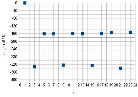
While not required by the script, in this case $c/d = 1/48,$ so each real DFT bin corresponds to a harmonic of the prototypical sinusoid. The fundamental frequency's amplitude measures as -1.75E-7 dBFS, the 5th harmonic as -160.90 dBFS and the 7th as -160.75 dBFS. Unfortunately I could not find a suitable multiple precision Fast Fourier Transform (FFT) library, but I think those three numbers came out in sufficient precision using NumPy's rfft. The precision is not sufficient to calculate the amplitude of say the 3rd harmonic seemingly at about -333 dBFS (Fig. 4).

Figure 4. Magnitudes of the real DFT bins of the quantized sequence of a synchronously sampled cosine with $A=2^{23}-1$, $f =$ 1000 Hz, and $f_s =$ 48 kHz. These results are only applicable when one of the samples is at the peak of the sinusoid, so not applicable to arbitrary phase shifts or asynchronous sampling.
With this $f/f_s$ the fundamental period is $L = 48$. The computed amplitudes of the harmonics are also correct for phase shifts of the prototypical cosine that are multiples of $2\pi/L$, because the cosine is sampled also at those phases, or such a multiple plus $\pi$, because of the symmetry properties of cosine. In the presented case the compatible phase shifts of the cosine are multiples of $7.5°$.
We have encountered here a troublesome combination of $L = 48$ and $A = 2^{23}-1$. We have samples $A\cos(8\times2\pi/L) =$ $A\cos(40\times2\pi/L) =$ $A/2$ and $A\cos(16\times2\pi/L) =$ $A\cos(32\times2\pi/L) =$ $-A/2$, and as $A$ happens to be an odd integer, those samples will always have a fractional part of $1/2$. The above reported amplitudes of the harmonics may thus be dependent on the rounding mode, or, the computation of the phase and/or evaluation of the cosine may have given a small numerical error which has determined the direction of rounding. This may even break the symmetry properties of the sequence, affecting which amplitudes of the harmonics of the period-$L$ frequency are zero.
Method validation
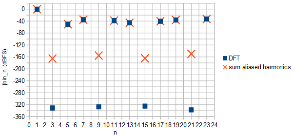
We can validate the two approaches against each other by choosing a pair of $A$ and $f/f_s$ that does not result in sampling of the quantized prototypical cosine at any of its discontinuities. Firstly, this removes having to choose arbitrarily which way a number exactly half-way between integers should be rounded, and secondly, should help in convergence of the infinite series in Eq. 6. Let's try $A = 8$ and $f/f_s = 1/48$. First, the real-DFT-based method, in Python:
import numpy as np
from sympy import Rational
def bins(A, c, d):
    L = Rational(d, np.gcd(c, d))  # Fundamental period (samples)
    waveform = np.around(A*np.cos(np.dot(range(L), 2*np.pi*c/d)))
    return np.fft.rfft(waveform)/(A*L/2)

A = 8  # amplitude (positive reals)
c = 1000  # numerator of f/f_s (positive integer)
d = 48000  # denominator of f/f_s (positive integer)
[20*np.log10(float(abs(x))) for x in bins(A, c, d)]  # real DFT magnitudes (dBFS)
This results in the following amplitudes of the harmonics, printed in precision beyond their accuracy, in dBFS:
-inf, 0.005622747208892056, -inf, -331.19944825653926, -inf, -50.41376796795221, -inf, -35.41599672115829, -inf, -327.2878768807577, -inf, -38.14783193548751, -inf, -45.42857299685606, -inf, -324.8188873214554, -inf, -40.41625528549065, -inf, -36.12873038111221, -inf, -337.55682735433885, -inf, -33.04816436790989, -inf
Then, aliasing the harmonics of the quantized prototypical cosine by evaluating Eq. 6, with the series truncated to the first approximately $10^4\pi A$ terms, continuing with the imports and constants of the previous Python script:
import mpmath as mp
def a_n(A, n):
    if int(n) & 1:
        return 4*mp.floor(A + 0.5)/(mp.pi*n)*mp.sin(mp.acos((mp.floor(A + 0.5)-0.5)/A)*n) + 4/(mp.pi*n)*mp.nsum(lambda k: k*( mp.sin(mp.acos((k-0.5)/A)*n) - mp.sin(mp.acos((k+0.5)/A)*n) ), [1, mp.floor(A + 0.5)-1])
    else:
        return 0

mp.mp.prec = 100
L = Rational(d, np.gcd(c, d))  # Fundamental period (samples)
if c == np.gcd(c, d):
    for n in range(L/2):
        bin = a_n(A, n) + mp.nsum(lambda k: a_n(A, k*L - n) + a_n(A, k*L + n), [1, int(10000*mp.pi*A)])
        float(20*mp.log10(mp.fabs(bin)/A)) # harmonic amplitude (dBFS)
else:
    print("Error: fundamental frequency must be in bin_1")

mp.mp.prec = 53
which results in the following amplitudes, printed in precision beyond their accuracy, in dBFS:
-inf, 0.005622452922818016, -inf, -165.35811090601203, -inf, -50.41370472648242, -inf, -35.41599394709451, -inf, -155.34167605811237, -inf, -38.14782298030069, -inf, -45.42859376902997, -inf, -164.6586753088176, -inf, -40.41623886311205, -inf, -36.12872396082294, -inf, -149.78722963456818, -inf, -33.04815743325275
The results seem to agree within their numerical accuracy (Fig 6.).

Figure 6. Comparison of amplitudes, in dBFS, of harmonics of a quantized cosine sampled synchronously, with $A = 8$ and $f/f_s = 1/48$, calculated by the real-DFT-based method (blue squares) and by summing coefficients $a_n$ of harmonics that alias to the same frequency (orange crosses).
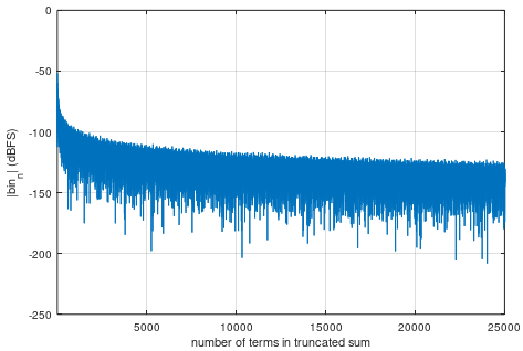
The 3rd harmonic amplitude calculated by truncating the sum in Eq. 6 converges very slowly as function of the number of terms (Fig. 6). This is probably the case also with the other low-amplitude harmonics. It does not seem feasible to reach the accuracy of the real-DFT-based method using the harmonic aliasing method.

Figure 7. $\operatorname{bin}_3$ as function of the number of terms in truncation of the sum in Eq. 6.
Synchronous sampling of a sinusoid of arbitrary phase with rational $f/f_s$
24-bit quantization
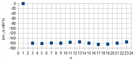
The real-DFT-based method is simple to modify for arbitrary phase shifts of the prototypical cosine. For $A = 2^{23}-1$, $f =$ 1000 Hz, $f_s =$ 48 kHz, and a phase shift $\phi = 0.123$ in radians, the amplitudes of the harmonics of the fundamental period can be computed by the following Python script:
import numpy as np
from sympy import Rational
def bins(A, c, d, phi):
    L = Rational(d, np.gcd(c, d))  # Fundamental period (samples)
    waveform = np.around(A*np.cos(np.dot(range(L), 2*np.pi*c/d) + phi))
    return np.fft.rfft(waveform)/(A*L/2)

A = 2**23-1  # amplitude (positive real)
c = 1000  # numerator of f/f_s (positive integer)
d = 48000  # denominator of f/f_s (positive integer)
phi = 0.123  # phase shift of the cosine (radians)
[20*np.log10(float(abs(x))) for x in bins(A, c, d, phi)]  # real DFT magnitudes (dBFS)

Figure 8. Magnitudes of the real DFT bins of the quantized sequence of a synchronously sampled cosine with phase shift $\phi = 0.123$, $A=2^{23}−1$, $f=$ 1000 Hz, and $f_s$= 48 kHz.
Asynchronous sampling of a sinusoid with rational $f/f_s$
Asynchronous sampling with rational $f/f_s$ can be modeled by assuming that $f/f_s$ is very close to a rational number. Then, locally the sequence of samples appears periodic with a computable harmonic spectrum. After sufficient time has elapsed, the phase of the prototypical sinusoid will have drifted to a different value and with a different local harmonic spectrum. For a random such sufficient time, the drift is a random variable between $0$ and $2\pi$. A reasonable probabilistic analog of the amplitude of a real DFT bin of the periodic sequence is the expected value of the square of its absolute value, $\operatorname{E}[|\operatorname{bin}_n|^2]$, which can be expressed in the same dBFS scale. We can estimate its value using uniform statistical sampling over phase shifts $\phi$ in a non-redundant range $0 < \phi < 2\pi/L$, where $L$ is the fundamental period of the locally periodic sequence. The end points of the range shall be deliberately left out so that we don't have the previously encountered problem with rounding modes and such.
24-bit quantization
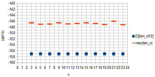
$\operatorname{E}[|\operatorname{bin}_n|^2]$ is estimated for $A = 2^{23}-1$, $f =$ 1000 Hz, and $f_s =$ 48 kHz, by the following Python script, which also estimates $\max|\operatorname{bin}_n|$ over random phase shifts, representing the worst-case non-fundamental harmonic amplitudes in the local spectra:
import numpy as np
from sympy import Rational
def E_sq_abs_bins_and_E_max_sq_abs_bins(A, c, d, N):
    L = Rational(d, np.gcd(c, d))  # Fundamental period (samples)
    num_bins = int((L + 2)/2)
    sum_sq_bins = np.zeros(num_bins)
    max_sq_bins = np.zeros(num_bins)
    for n in range(N):
        phi = float((0.5 + n/N)*2*np.pi/L)
        waveform = np.around(A*np.cos(np.dot(range(L), 2*np.pi*c/d) + phi))
        sq_bins = np.square(np.absolute(np.fft.rfft(waveform)/(A*L/2)))
        sum_sq_bins = sum_sq_bins + sq_bins
        max_sq_bins = np.maximum(max_sq_bins, sq_bins)
    return [sum_sq_bins/N, max_sq_bins]

A = 2**23-1  # amplitude (positive real)
c = 1000  # numerator of f/f_s (positive integer)
d = 48000  # denominator of f/f_s (positive integer)
N = 2**18 # size of statistical sample (positive integer)
results = E_sq_abs_bins_and_E_max_sq_abs_bins(A, c, d, N)
[10*np.log10(float(x)) for x in results[0]]  # est. expected value of real DFT squared magnitudes (dBFS)
[10*np.log10(float(x)) for x in results[1]]  # est. max real DFT squared magnitudes (dBFS)
The results convergence quite slowly as the size of the statistical sample N is increased, and the accuracy requirements stated in the question are almost but not quite fulfilled by a day's calculation on my PC for $\operatorname{E}[|\operatorname{bin}_n|^2]$ and not at all for $\max|\operatorname{bin}_n|$. In the results obtained (Fig. 9) $\operatorname{E}[|\operatorname{bin}_n|^2]$ is about -157.1 dB and $\max|\operatorname{bin}_n|$ about -147.2 to -146.0 dBFS for non-fundamental harmonics. For the fundamental frequency, $\operatorname{E}[|\operatorname{bin}_1|^2]$ is in the order of -0.95E-11 dBFS, and $\max|\operatorname{bin}_1|$ is in the order of 3.4E-7 dBFS or higher.

Figure 9. Estimated $\operatorname{E}[|\operatorname{bin}_n|^2]$ (blue squares) and $\max|\operatorname{bin}_n|$ (red lines) for local $\operatorname{bin}_n$ in slow-drifting asynchronous sampling, for $A = 2^{23}-1$, $f =$ 1000 Hz, and $f_s =$ 48 kHz, estimated by a uniform statistical sample of phase shifts with a sample size of $2^{18}$.
The estimates show that asynchronous sampling gives a smoothing effect on the statistics of the local amplitudes of the harmonics, compared to synchronous sampling with a fixed alignment of the prototypical cosine with respect to the sampling grid. However, with asynchronous sampling, sometimes the worst case local harmonic peaks occur, whereas with synchronous sampling the harmonic amplitudes are well controlled and the worst cases are avoided by a suitable choice of phase shift.
Asynchronous sampling of a sinusoid with rational $f/f_s$ in the limit $L/A\to 0$
In this section of the answer, we will consider only the question's case that $L$ is even and $f/f_s = 1/L$, that is to say that $\operatorname{bin}_1$ corresponds to the frequency of the prototypical sinusoid.
If the length of the fundamental period of the locally periodic sequence of samples $L$ calculated by Eq. 4 is very small compared to the amplitude $A$ of the prototypical sinusoid, then for different phase shifts of the sinusoid, the quantization error can perhaps be considered a sequence of independent pseudorandom numbers distributed uniformly from -0.5 to 0.5, with an antiperiodicity constraint if $L$ is even (and some other constraint if $L$ is odd). Independence of the quantization errors would require that at a number of certain small time lags the autocorrelation of the quantized prototypical sinusoid approaches zero, but this is not something we know to be a fact. If it was true, then in the limit $L/A \to 0$ any sequence consisting of ±0.5's could be found as a quantization error sequence at some phase shift $\phi$ of the prototypical cosine, and within those sequences there would be sequences that maximize $|\operatorname{bin}_n|$ of the real DFT of the quantization error sequence. Due to orthogonality of the real DFT basis vectors, if $n$ does not correspond to the fundamental frequency of the sinusoid, then $\operatorname{bin}_n$ of the quantized sequence equals $\operatorname{bin}_n$ of the quantization error. If $n$ corresponds to the fundamental frequency, then $\operatorname{bin}_n$ of the quantized sequence equals $\operatorname{bin}_n$ of the quantization error plus $Ae^{i\phi}$.
Even if we do not assume independence of quantization errors, we can use the line of thinking of the previous paragraph to find an upper bound of $\max|\operatorname{bin}_n|$, the maximum absolute bin value for a harmonic of the prototypical sinusoid. A worst-case sequence of ±0.5's that maximizes $|\operatorname{bin}_n|$ could be found by an exhaustive search in the binary sequences, but can also obtained directly. A worst-case sequence is any sequence $\operatorname{seq}_k = 0.5\operatorname{sgn}\big(\cos(2\pi nk/L + \chi)\big)$, where $\operatorname{sgn}$ is the sign function, and with a phase shift $\chi$ that does not result in a zero crossing of the expression's sinusoid being at any sample point (the integers). One worst-case sequence is found in the limit of approaching from one side the transition between two worst-case sequences:
$$\begin{eqnarray}\operatorname{seq}_k &=& 0.5\times\begin{cases}\operatorname{sgn}\big(\sin(2\pi nk/L)\big),&\text{if }\sin(2\pi nk/L) \ne 0,\\
\cos(2\pi nk/L),&\text{if }\sin(2\pi nk/L) = 0,\end{cases}\\
&=& 0.5\times\begin{cases}\operatorname{sgn}\big(\sin(2\pi nk/L)\big),&\text{if }2kn \text{ mod } L \ne 0,\\
\cos(2\pi nk/L),&\text{if }2kn \text{ mod } L = 0,\end{cases}\end{eqnarray}\tag{7}$$
where $\text{ mod }$ denotes remainder in integer division in a numerically safe expression. An upper bound of $\max|\operatorname{bin}_n|$ is then found by real DFT of the worst-case sequence.
24-bit quantization
For odd $n$ the sequence given by Eq. 7 satisfies the antiperiodicity constraint for even $L$, and we can calculate an upper bound of $\max|\operatorname{bin}_n|$ of the maxima of local harmonic amplitudes $|\operatorname{bin}_n|$ for $A = 2^{23}-1$, $f =$ 1000 Hz and $f_s =$ 48 kHz, in Python:
import numpy as np
from sympy import Rational
def bins_max_err_seq(A, c, d, n):
    L = int(Rational(d, np.gcd(c, d)))  # Fundamental period (samples)
    waveform = 0.5*np.sign(np.sin(np.dot(range(L), 2*np.pi*n/L)))
    for k in range(L):
        if 2*k*n % L == 0:
            waveform[k] = 0.5*np.cos(k*2*np.pi*n/L)
    return np.fft.rfft(waveform)/(A*L/2)

A = 2**23-1  # amplitude (positive real)
c = 1000  # numerator of f/f_s (positive integer)
d = 48000  # denominator of f/f_s (positive integer)
if c == np.gcd(c, d) and int(Rational(d, np.gcd(c, d))) % 1 == 0:
    for n in np.arange(1, int(d/c/2 + 1), 2):
        print(str(n) + "," + str(20*np.log10(float(abs(bins_max_err_seq(A, c, d, n)[n])))))  # real DFT magnitude of bin n for the maximum quantization error sequence (dBFS)
else:
    print("Error: Fundamental frequency must be in bin 1 and L must be even\n")
For the odd harmonics, for $A = 2^{23}-1$, $f =$ 1000 Hz and $f_s =$ 48 kHz, we get locally $\max|\operatorname{bin}_n| \le $ -142.34 dBFS when the number of the harmonic $n$ is divisible by 3, and $\max|\operatorname{bin}_n| \le $ -142.39 dBFS otherwise which applies to the 5th and to the 7th harmonic. This seems compatible with Fig. 9, with an about 4 dB higher upper bound of the maximum local amplitudes of harmonics compared to the maximum local harmonic amplitude found by numerical search in actual quantization error sequences. A willing eye can also see an elevation in $\max|\operatorname{bin}_n|$ of Fig. 9 when $n$ is divisible by 3.
This answer has reached the maximum allowed length of 30000 characters.

