Is there such a thing as band-limited non-linear distortion?

Question

So if you generate a square wave by just switching a signal between two values, at sample boundaries, it produces an infinite series of harmonics, which alias and produce tones below your fundamental, which is very audible. The solution is Band-Limited Synthesis, either using additive synthesis or band-limited steps to produce waveforms that are the same as if you had band-limited the ideal mathematical square wave before sampling it:

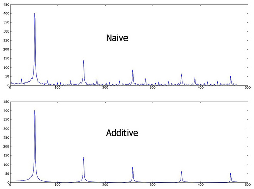
http://flic.kr/p/83JMjT

But I just realized that if you apply large amplification to a digital sine wave and then clip it digitally, it will produce the same square wave shape, without the Gibbs phenomenon ripples. So it's then also producing aliased distortion products, right? So any non-linear distortion in the digital domain that produces harmonics outside of the Nyquist limits will produce aliased distortion products? (Edit: I've done some tests and confirmed that this part is true.)

Is there such a thing as band-limited distortion, to simulate (in the digital domain) the effects of distorting (in the analog domain) before band-limiting and sampling? If so, how do you do it? If I search for "bandlimited distortion" I find some references to Chebyshev polynomials, but I don't know how to use them or if they only work for sine waves or what:

This instrument does not attempt to generate band-limited distortion. Those interested in band-limited distortion should investigate the use of Chebyshev polynomials to generate the effect. Hyperbolic Tangent Distortion

 

"Chebyshev polynomial" -- shaping functions with the important property that they are intrinsically band-limited i.e. they do not introduce spurious spectral harmonics due to overlapping etc. Wave Shaper

Answer 1

Applying a non-linear function will always introduce harmonics, and mixing non-linear functions with sampled versions of continuous signals does add the wrinkle you note above (where high-frequency harmonics are aliased to low frequencies.)

I can think of a few ways to proceed:

1. You can use an oversampling factor high enough to capture the extra harmonics (up to some arbitrary precision, e.g. your noise floor),
2. You can use a "softer" clipping function (see, for example, here) that has harmonics that die out sooner than the hard clipper. This is easier to model, but introduces its own distortion at low frequencies.
3. Building on the approach you suggested above, interpolate your sampled signal (e.g. using a Lagrange or Chebyshev interpolator) to construct a continuous-time model. Then, apply the hard clipper and low-pass in a simulated continuous-time domain. Sample the result.

You can combine (1) and (2). The third approach is complex, but gives you the best control over how much distortion to admit, and will probably scale better to very high fidelity requirements.

For non-linear functions that admit a series expansion (e.g. Taylor/Maclaurin), you can get a decent intuition for how fast the harmonics decay. The Maclaurin expansion of a function $f(x)$ is:

$$f(x)=\sum_{n=0}^\infty \left[ \frac{f^{(n)}(0)}{n!} x^n\right]$$

In your case, $f(x)$ is the clipping function. (You can't do this with a hard clipper, at least not naively!) If you consider the substitution $x=g(t)$, where $g(t)$ is your input signal, the $x^n$ becomes $g(t)^n$, which you can consider to be the convolution of your input signal with itself $n$ times. Thus, for low-pass signals, the $n$th term of the infinite summation has a bandwidth $n$ times that of your signal. To complete the picture, you need to figure out the amplitude associated with each term and decide how many terms in the summation are relevant.

(With a little thought, you might also be able to use this form directly to approximate the filtered non-linearity. That would require a good series representation for the clipper.)

Answer 2

A few approaches to alias-free nonlinear distortion (in increasing order of difficulty):

1. Subband distortion: Use a low pass filter to extract the lower end of the signal. If you choose a cutoff frequency of $\frac{f_s}{2N}$ you can apply any non-linear transfer function $f$ with derivatives starting at $f^{N+1}$ vanishing to avoid aliasing. Add just the distortion output of the low band back to the original signal. For this, modify your nonlinear transfer function to only produce the distortion, not the incoming signal. This approach is often totally sufficient for audio, because the distortion contribution of the higher frequencies would be inaudible in most cases.

2. Oversampling: This is similar to approach 1, but does require the extra steps of upsampling and downsampling to make sure that all information in the original signal band contributes to the distorted signal, if you think this is needed. It also allows you to distort to higher order, because parts of the back-folded spectrum will be removed by the downsampling filter. That means if you oversample by a factor $N$, the derivatives of the nonlinear transfer function starting at order $2N$ have to vanish. The procedure is a simple as upsampling, applying the nonlinear transfer function, downsampling.

3. Using a local analytic solution: Any smooth nonlinear transfer function can be applied to a signal that is described by a power series. If you let the transfer function act on a power series, you will get a power series back. If you restrict yourself to truncated power series of a certain order, and the transfer function to a certain degree of smoothness, you can write the transfer function as a map on the coefficients of the truncated series. That means instead of $f:\mathbb{R}\to\mathbb{R}$, you consider $f:\mathbb{R}^N\to\mathbb{R}^M$ taking an input series expansion of length $N$ to an output series expansion of length $M>N$. With this understanding, you can use a local finite approximation of the input signal in terms of a power series and map it to a power series approximation of the output. Then you can analytically integrate the output series to create a box-car antialiasing filter to get the output sample value. All these computations can be done symbolically, and because you have to include local features of the input signal, you will finally get a nonlinear filter that uses past values of your input signal to generate the current output.

4. Constrain based algebraic design: In the previous item, you have seen that antialiasing nonlinear distortion leads to nonlinear filters. Of course, not all nonlinear filters are alias free, but some may be. So the obvious question is for a criterium to make such a filter strictly alias free and how to design it. As it turns out, an equivalent statement to being free of aliasing is, that the non-linear filter commutes with sub-sample translations. So you must make sure that it does not make a difference if you translate first and then filter, or filter first and then translate. This condition leads to very strict design constraints for nonlinear filters, but depends on how you realise the signal translation. For example, the ideal translation would require infinitely many coefficients for the nonlinear filter. So you have to approximate signal translation to finite order to get a finite nonlinear filter. Alias-freeness scales with the approximation you use, but you have very good control over it. After you've worked through the mathematics of this approach, you can design any (not just smooth) nonlinear transfer function as a nearly ideal digital model in the form of a nonlinear filter. I cannot possibly sketch the details here, but maybe you can find some inspiration from this description.

Answer 3

One algorithm that qualifies as bandlimited distortion is the use of Chebyshev polynomials with sinusoidal inputs for waveshaping synthesis. The Chebyshev polynomials [of the first kind] can be defined as $$ T_n(x) = \mathrm{cos}(n \, \mathrm{arccos}(x)). $$

I won't go into details here, but there's a relatively simple derivation using De Moivre's Theorem which shows how the above formula defines a set of polynomials (cf. Sec. 7.2 in Digital Filters by Hamming). The trigonometric definition is useful because it makes it easy to see how each $T_n(x)$ maps a unit amplitude cosine into its nth harmonic, i.e.

$$ T_n(\mathrm{cos}(kx)) = \mathrm{cos}(n\,\mathrm{arccos}(\mathrm{cos}(kx))) = \mathrm{cos}(nkx). \tag{1} $$

The polynomials themselves can be easily generated by using the following recurrence relation:

$$ T_0(x) = 1 \\ T_1(x) = x \\ T_n(x) = 2x\,T_{n-1}(x) - T_{n-2}(x). $$

Here are the first few:

$$ \eqalign{ T_0(x) &= 1 \\ T_1(x) &= x \\ T_2(x) = 2x(x - 1) &= 2x^2 - 1 \\ T_3(x) = 2x(2x^2 - 1) - x &= 4x^3 - 3x \\ T_4(x) = 2x(4x^3 - 3x) - (2x^2 - 1) &= 8x^4 - 8x^2 + 1 \\ \ldots } $$

Another way to gain intuition for property $(1)$ is to consider, for example, the operation of $T_2$ on the complex exponential form of $\mathrm{cos}(x)$

$$ \eqalign{2\,\mathrm{cos}^2(x) - 1 &= 2\left(\frac{e^{ix} + e^{-ix}}{2}\right)^2 - 1 \\ &= \frac{2}{4}(e^{i2x} + 2e^{ix}e^{-ix} + e^{-i2x}) - 1 \\ &= \left(\frac{e^{i2x} + e^{-i2x}}{2}\right) + \frac{2}{2} - 1 \\ &= \mathrm{cos}(2x). } $$

By computing a Chebyshev Series

$$ f(x) = \sum_{n = 0}^{\infty}{a_n\,T_n(x)} $$

truncated to an appropriate value of $n$, you get a waveshaper (i.e. $f(x)$) that, when applied to a unit amplitude cosine, will generate an arbitrary [integer] set of bandlimited harmonics.

Answer 4

@robert-bristow-johnson explains this very clearly on comp.dsp:

you have to oversample to a finite extent. if you represent the (memoryless, i assume) non-linearity as a finite order polynomial (that approximates whatever curve you are trying to implement), then whatever is the order of polynomial is the same factor of oversampling needed and no aliases will occur. then low-pass filter (at that oversampled rate) to get rid of all frequency components higher than your original Nyquist, then downsample and you will not have aliasing.

In other words, if your nonlinearity is a polynomial, the highest frequency that can be produced by the distortion will be the highest frequency in your signal times the order N of the polynomial. (The polynomial nonlinearity is multiplying the signal by itself N times, so its spectrum gets convolved with itself and spreads out by the same ratio.)

So then you know the maximum frequency (whether Nyquist or some lower limit for your application), and you know the order of the polynomial, so you can oversample enough to prevent aliasing, do the distortion, and then low-pass filter and downsample.

In fact, you can reduce the oversampling rate by letting some aliasing happen, as long as it's contained in the band that will be removed before downsampling:

another little trick is that you need not care about aliasing that folds down to the area that you'll LPF out. so a 5th order polynomial needs only to have an oversampling ratio of 3. those top 2 harmonics might alias, but won't get back into the baseband. when downsampling, you filter those aliased harmonics out. so i think the hard and fast rule is

oversampling ratio = (polynomial order + 1)/2