3
$\begingroup$

I'd like to reproduce results from this paper in which the authors used Group Delay-grams as an input to the Machine Learning model. The Machine Learning side is not the one that I have problems with. I have a problem with computing a Group Delay function of an audio file.

To begin with, I know that a group delay per se is a property of the filter. Authors of the paper, however, wrote something like this

Group delay [10] is defined as the negative derivative of the phase spectrum of STFT: $$\tau(\omega,t)=-\frac{d(\theta(\omega,t))}{d\omega}\quad(2)$$ As the implementation of Equation (2) requires the unwrap- ping of the phase spectrum, the group delay function can be alternatively calculated using only the amplitude values: $$\tau(\omega,t)=\frac{X_{R}(\omega,t)Y_{R}(\omega,t)+Y_{I}(\omega,t)X_{I}(\omega,t)}{|X(\omega,t)|^2}\quad(3)$$ where $R$ and $I$ denote the real and imaginary parts. $X(\omega,t)$ and $Y(\omega,t)$ denote the STFT of $x(n)$ and $nx(n)$, respectively.

This, I believe, is supposed to generate an image like in Fig. 3 in the paper, which looks like this (after either truncating or padding to the length of 256 along the time axis)

enter image description here

The problem is that when I try to compute this GD-gram from the equation above, the matrices multiplication cannot be done since both $X$ and $Y$ are non-symmetric. This is the original paper, that is referenced in both this paper and [10], where the authors are deriving the equation (3).

As I understood, the matrices multiplication is a standard one, not element-wise (element-wise multiplication doesn't produce the result that is in the paper). In my implementation below I'm using a window of length 800 samples since the authors of the paper use 50 ms window, which corresponds to 800 samples for 16 kHz sampling rate audio file. I tried to implement that in python as follows:

from scipy.io import wavfile
from scipy.signal import stft, get_window
import numpy as np
import matplotlib.pyplot as plt

rate, data = wavfile.read("test.wav")

n_data = np.multiply(data, np.arange(len(data)))
f, t, X = stft(data, rate, window="hamming", nperseg=800, return_onesided=False)
f_n, t_n, Y = stft(n_data, rate, window="hamming", nperseg=800, return_onesided=False)
group_delay = (np.dot(X.real, Y.real) + np.dot(Y.imag, X.imag)) / np.power(np.abs(X), 2)

but the code fails with

---------------------------------------------------------------------------
ValueError                                Traceback (most recent call last)
<ipython-input-8-0058b9785caf> in <module>
----> 1 group_delay = (np.dot(X.real, Y.real) + np.dot(Y.imag, X.imag)) / np.power(np.abs(X), 2)

ValueError: shapes (800,109) and (800,109) not aligned: 109 (dim 1) != 800 (dim 0)

which is rather obvious. I tried to implement that in Matlab as well, hoping that maybe it's a python fault but it fails as well.

[x,fs] = audioread('test.wav');
n_x = x .* [1:size(x,1)];
X = spectrogram(x, 800, 400, 2048, fs);
Y = spectrogram(n_x, 800, 400, 2048, fs);
T = (real(X) * real(Y) + imag(Y) * imag(X)) / abs(X)^2;

How can I compute the Group Delay function using mentioned equation

$\endgroup$
10
  • $\begingroup$ The element-wise multiplication is what is happening in (3), not matrix multiplication. $\endgroup$
    – Peter K.
    Commented Dec 17, 2018 at 16:31
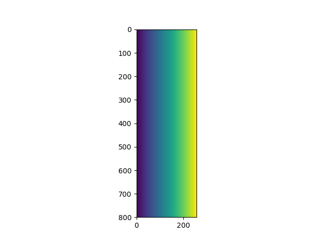
  • $\begingroup$ I thought that is the case, but after performing the element-wise multiplication and plotting the resulting matrix I obtain different results. The image that I included in the question somewhat resembles STFT itself. The image that you get When performing element wise multiplication looks like Simple gradient from Left to right which makes sense since Y is the STFT of nx(n) $\endgroup$
    – Colonder
    Commented Dec 17, 2018 at 16:36
  • $\begingroup$ Nothing in the paper suggests matrix multiplication. The equation is explicitly saying element-wise multiplication because it is indexed by $\omega$ and $t$, so all the terms are scalars. $\endgroup$
    – Peter K.
    Commented Dec 17, 2018 at 16:38
  • $\begingroup$ @Colonder, sorry to bother. Can you reproduce the result of this paper? I've tried to implement reference CNN with group delay, but the eer of first stage was about 30%, which should be about 12% according to the paper. I wonder if i missed something. $\endgroup$
    – Haojun
    Commented Jan 2, 2019 at 2:58
  • $\begingroup$ @Haojun I'm working on that, will let you know if I will get anything $\endgroup$
    – Colonder
    Commented Jan 9, 2019 at 20:30

1 Answer 1

5
$\begingroup$

The problem is that the stft function is splitting the signal up into different windows. That means that the signal from time $n$ to $n+N_{w}-1$ is multiplied by $$ n, n+1, n+2, \ldots, n+N_w-1$$ instead of $$ 0, 1, 2, \ldots, N_w-1 $$ which is causing the scaling problem.

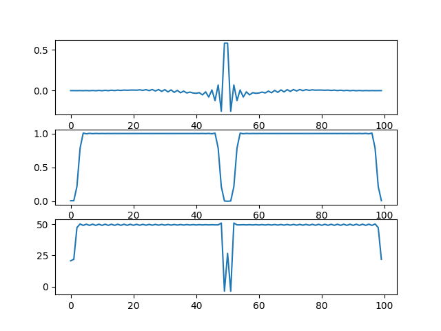
If I apply the group delay calculation from this derivation, I get:

enter image description here

where the top plot is the "data", the middle plot is the FFT of the data, and the bottom plot is the group delay. The group delay plot seems to be correct ($\tau_g = 49.5$, except for where the data is zero in the frequency domain.

To get this to work with the stft function, you're going to have to modulate the data with a sawtooth function rather than just np.arange(len(data)).

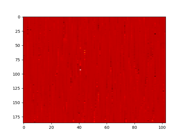
If I slice the sound file bachfugue.wav using the new, new code below I get the following image, which is more like what I'd expect.

Group Delay image


New New Code Below

#!/opt/local/bin/python2.7
from scipy.signal import firwin
import numpy as np
import matplotlib.pyplot as plt
from scipy.io import wavfile


def group_delay(sig):
    b = np.fft.fft(sig)
    n_sig = np.multiply(sig, np.arange(len(sig)))
    br = np.fft.fft(n_sig)
    return np.divide(br, b + 0.01).real


rate, data = wavfile.read('bachfugue.wav')

N_w = 1024
L = np.floor(len(data)/N_w).astype(int)

full_delay = np.zeros((L, N_w))
for index in range(L):
    window = data[index:(index+N_w), 1].astype(float)
    full_delay[index][:] = group_delay(window)

plt.imshow(full_delay[0::10, 0::10], cmap=plt.get_cmap('hot'),aspect='auto')
plt.show()

New Code Below

#!/opt/local/bin/python2.7
from scipy.signal import firwin
import numpy as np
import matplotlib.pyplot as plt


N = 100
data = firwin(N, [0.05, 0.95], width=0.05, pass_zero=False)
n_data = np.multiply(data, np.arange(len(data)))
rate = 1

B = np.fft.fft(data)
Br = np.fft.fft(n_data)
group_delay2 = np.divide(Br, B + 0.01).real

plt.figure(1)
plt.subplot(311)
plt.plot(data)
plt.subplot(312)
plt.plot(np.abs(B))
plt.subplot(313)
plt.plot(group_delay2)

plt.show()

--

Original Answer

I've implemented it as I think it should be. I don't have your data, so I've just made a sinusoid.

The resulting plot is below. Code at end.

So I'm wondering what you should expect to see... more thought needed. I'll read that paper in more detail and see what I can make of it.

enter image description here


Now that I've had a chance to read through it, I'm wondering if that is correct. Based on this derivation... I think the real way to do it might be different. I'll try to code that up later.


Python Code

#!/opt/local/bin/python2.7
from scipy.signal import stft
import numpy as np
import matplotlib.pyplot as plt

N = 102400
rate = 1.0
data = []
for phi in ([2.0*3.14159265*x for x in range(0, N-1, 1)]):
    data.append(np.sin(phi))

n_data = np.multiply(data, np.arange(len(data)))
f, t, X = stft(data, rate, window="hamming", nperseg=800, return_onesided=False)
f_n, t_n, Y = stft(n_data, rate, window="hamming", nperseg=800, return_onesided=False)
# group_delay = (np.dot(X.real, Y.real) + np.dot(Y.imag, X.imag)) / np.power(np.abs(X), 2)

group_delay = np.divide(np.multiply(X.real, Y.real) + np.multiply(Y.imag, X.imag), np.power(np.abs(X), 2))

plt.imshow(group_delay)
plt.show()
$\endgroup$
5
  • 1
    $\begingroup$ This is what I obtained earlier as well. I think, though, that the result resembles nowhere near the image from the paper. $\endgroup$
    – Colonder
    Commented Dec 18, 2018 at 10:05
  • $\begingroup$ @Colonder Yes, my attempt at the example in my edit gives the same result. Not sure what's going on there.... More thought needed. Watch this space. $\endgroup$
    – Peter K.
    Commented Dec 18, 2018 at 13:27
  • $\begingroup$ @Colonder I believe that solves your problem. $\endgroup$
    – Peter K.
    Commented Dec 18, 2018 at 14:59
  • $\begingroup$ could you try to apply your new code to some wav audio file? It can be whichever you want, doesn't matter $\endgroup$
    – Colonder
    Commented Dec 18, 2018 at 21:37
  • $\begingroup$ @Colonder See edit. I think that's what you need. $\endgroup$
    – Peter K.
    Commented Dec 19, 2018 at 2:37

Not the answer you're looking for? Browse other questions tagged or ask your own question.