INTUITIVE EXPLANATION
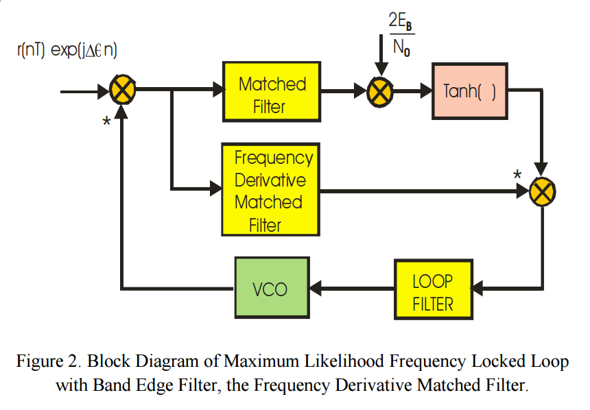
This is very similar in form (as a maximum likelihood detector in both cases) to Timing Error Detectors, where instead of a "Frequency Derivative Matched Filter", A "Time Derivative Matched Filter" is used.
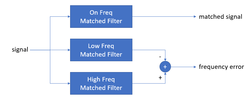
We could instead implement this Frequency Lock Loop with 3 match filters. This will be easy to see if we first consider the simpler case with no modulation, and show how a frequency error metric can be derived as depicted in the diagram below:

The matched filters consist of an "On Frequency Matched Filter", which has coefficients matched to the waveform assuming there is no frequency offset. The other two are the same coefficients frequency translated slightly up and down in frequency. The resulting output of each matched filter is what we can expect to see out of any one of the filters as a frequency error is introduced in the signal. The matched filter output is maximum when the signal is aligned in frequency with the filter, and goes down according to a frequency shift (as well as changes in phase). We could using three filters as shown, establish a frequency error metric by simply subtracting the outputs of the Low and High Matched Filters. This is synonymous with an Early-Late Timing Discrimator used in timing recovery applications, where instead three matched filter are used with a "Prompt" and then an "Early" and "Late" that are positioned forward and backward in time.
The difference between the two filter outputs is an approximation of a derivative! (So if the filters are shifted in frequency, it is a frequency domain derivative; and similarly in the Early-Late timing recover, the Early-Late is an approximation of a time domain derivative!).
So instead of the complexity of two filters each for the Low and High frequency cases, we can instead use a single filter which has the frequency domain derivative of the "On Freq Matched Filter". This results in a beautiful "S-curve" discriminator producing an output proportional to frequency error.
Under case of modulation, this frequency error term will also be modulated, and the complex conjugate product serves to strip the modulation from the error term for the loop.
The scaling by the SNR and hyberbolic tangent is the maximum liklihood optimization as further explained below.
MORE DETAILED ANALYTICAL EXPLANATION
The conjugate product of the two filters form a frequency discriminator with an error output that is proportional to a frequency offset at the input.
This is due to the relationship that the cross correlation in one domain is the conjugate product in the other domain (you can skip past the derivation unless interested):
$$c(\tau) = XCORR[x(t)y(t)]$$
$$c(\tau) = \int_{t=-\infty}^{\infty}x^*(t)y(t+\tau)dt$$
$$C(\omega) = \mathscr F\{y(t)\}= \int_{\tau=-\infty}^{\infty}\bigg[\int_{t=-\infty}^{\infty}x^*(t)y(t+\tau)dt\bigg]e^{-j\omega \tau}d\tau$$
$$=\int_{t=-\infty}^{\infty}x^*(t)\bigg[\int_{\tau=-\infty}^{\infty}y(t+\tau)e^{-j\omega \tau}d\tau\bigg]dt$$
From the shift property of the Fourier Transform, the terms inside the brackets are:
$$\int_{\tau=-\infty}^{\infty}y(t+\tau)e^{-j\omega \tau}d\tau = Y(\omega)e^{j\omega t}$$
Therefore:
$$C(\omega) =\int_{t=-\infty}^{\infty}x^*(t)\bigg[Y(\omega)e^{j\omega t}\bigg]dt$$
$$ = Y(\omega)\int_{t=-\infty}^{\infty}x^*(t)e^{j\omega t}dt = Y(\omega)\bigg[\int_{t=-\infty}^{\infty}x(t)e^{-j\omega t}dt\bigg]^*$$
$$ =Y(\omega)X^*(\omega) $$
The above shows that the cross correlation of two functions x(t) and y(t) in the time domain is equivalent to the conjugate multiplication of their Fourier Transforms (in the frequency domain). Similarly, and this is the important point to explaining the operation of the frequency discriminator, is that the converse is also true: the cross correlation of two functions in the frequency domain is equivalent to the conjugate multiplication of the transform of the same two functions in the time domain.
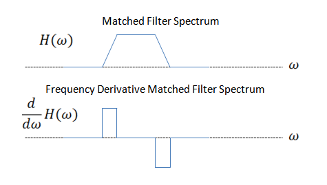
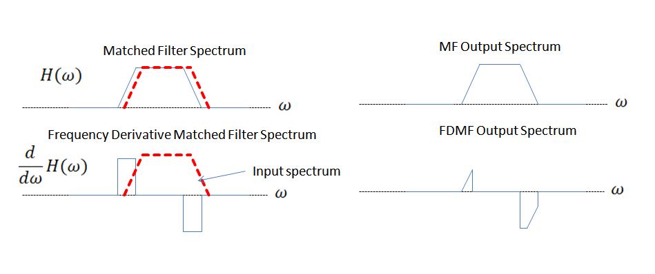
Consider the following as example spectrums of the "Matched Filter" and "Frequency Derivative Matched Filter" in the block diagram given by the OP. Notably the Frequency Derivative Matched Filter is a Band-Edge Filter.

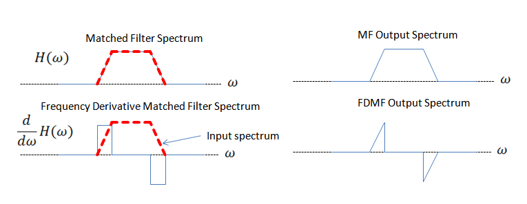
When there is no frequency error, the input spectrum would be aligned with both of these resulting in the following spectrums at the outputs of these filters. Notably, observe that cross-correlating these two output spectrums will result in a zero result specifically due to the positive and negative balance in the Frequency Derivative Matched Filter Spectrum!

If it helps to visually see how this can be the case (assuming familiarity with graphically doing convolution), consider how convolution and cross-correlation are related by complex conjugate and a mirroring of the spectrum:
Cross Correlation in the frequency domain:
$$C(\omega_\Delta) = \int_{t=-\infty}^{\infty}X^*(\omega)Y(\omega+\omega_\Delta)d\omega$$
Convolution in the frequency domain:
$$X(\omega) \ast Y(\omega) = \int_{t=-\infty}^{\infty}X(\omega)Y(-\omega+\omega_\Delta)d\omega$$
Thus we can use convolution to perform cross-correlation if we complex conjugate one of the waveforms, and reverse the other. We can see through graphical convolution how the result is zero if we were to convolve the complex conjugate of the matched filter spectrum with the mirrored derivative spectrum, when the spectrum is balanced as shown.
When there is a positive frequency error in the input signal as depicted in the graphic below, the input spectrum would be offset by the frequency error resulting in the following spectrums at the output of the two filters. In this case specifically, the cross-correlation of the two output spectrums would result in a negative value corresponding to the frequency error. Similarly a negative frequency error would result in a positive output value after the cross-correlation in frequency of the two spectrums.

The above shows how the cross-correlation of a Matched Filter Spectrum and a Frequency Derivative Matched Filter Spectrum results in an output value that is the error term for a frequency discriminator. Additionally we showed that cross-correlation in frequency is equivalent to the complex conjugate multiplication in time. Thus the complex conjugate multiplication of the two filters in the block diagram form a frequency discriminator as the error signal into the loop.
The frequency discriminator would operate as described without the scaling by the Signal to Noise Ratio (SNR) and Tanh() operation.
The additional scaling by the SNR, and the Tanh() operation are done to perform maximum likelihood frequency estimation (MLE). This shows the ideal implementation (in a maximum likelihood sense) but to my understanding the SNR scaling is rarely done in practice (but could be if an SNR estimation is performed as part of the receiver operation), and the Tanh() operation is typically approximated with a piecewise linear operation to be the signal for the small signal case when the signal is less than ±1 or limited to the sign of the signal (+1/-1) otherwise. So basically this path in the block diagram is hard limited for better performance with a limit that is dependent on the SNR of the received signal (a SNR dependent hard limiter is a typical operation within MLE implementations).
I believe that fred harris (fh) points out an advantage to this approach is how the derivative matched filter response is concentrated at the band edge where as we see through the convolution operation most of the information regarding frequency offset resides (when using a complex conjugate multiplier as a discriminator). The filter naturally blanks out the center portion of the spectrum which is not contributing further to the frequency error answer but would be contributing noise otherwise. Other advantages to this approach are that the symbol timing clock (timing recovery) can also be derived. I have not studied it personally in detail nor implemented this approach, but I believe fh makes the case that this implementation results in much lower pattern noise versus other carrier recovery (and timing recovery) approaches.

