variability among signals

Question

I have a set of $n$ low frequency time-varying signals $y(t)$.

I would like to express the variability within this set of signals using a single number. My current idea is to:

1. Compute the average signal $\bar y(t)$ for the set using

   $$\bar y(t) = \dfrac{y_1(t) + y_2(t) + \ldots + y_n(t)}{n} $$

2. Compute the 'standard deviation' of each individual signal with respect to the mean signal $\bar y$ using the Pearson correlation $r$

   $$\bar r = \dfrac{ r(y_1(t), \bar y(t)) + r(y_2(t), \bar y(t)) + \ldots + r(y_n(t), \bar y(t))}{n}$$

This would then give me a sense of the variability within the set of signals.

My question is whether there are better, different, or more established ways of doing this?

Answer 1

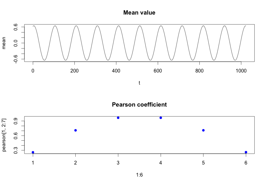
As an example of what I mean, let's have a look at a simple sinusoid (though I see you're actually assuming double gamma functions; I may rework this later to use those).

This models the signals as: $$ y_p(t) = \sin(\omega t + \phi_p) $$ so the only difference between them is the phase $\phi_p = (p-1)\pi/6$.

The top plot is the mean signal $\bar{y}(t)$ and the bottom plot shows the Pearson coefficient between $\bar{y}$ and $y_p$ for $p=1\ldots 6$ (so $n=6$).

As you can see, the Pearson coefficient varies quite widely even in this simple example.

---

R Code Below

# 26438

Nsigs <- 6
T<- 1024
omega <- 2*pi*0.00982734982
t <- 0:(T-1)

y <- matrix(,nrow = T, ncol = Nsigs)
phi <- c(0, 1*pi/6, 2*pi/6, 3*pi/6, 4*pi/6, 5*pi/6 )

for (idx in 1:Nsigs)
{
  #phi[idx] <- runif(1)*2*pi
  y[,idx] <- sin(omega*t + phi[idx])  
}

mean <- rowSums(y) / Nsigs

total <- matrix(,nrow = T, ncol = Nsigs+1)
total[,1] <- mean
total[,2:(Nsigs+1)] = y

pearson <- cor(total,use="complete.obs", method="pearson")

par(mfrow=c(2,1),pty="m")
plot(t,mean, type="l")
title("Mean value")

plot(1:6, pearson[1,2:7], pch=19, col="blue")
title("Pearson coefficient")

Answer 2

Compute the matrix Mij = [ y_i(t) y_j(t) ], where 0 <= i < n and 0 <= j < n. This matrix Mij will approximate a gain times the identity matrix when the signals are perfectly uncorrelated. So I suppose you could use sum of squares of the deviation from the gain times the identity matrix as a norm.