Find highest frequency of a very manky signal

Question

I'm trying to compute the highest frequency (as can be sampled) in some pretty manky looking discrete time-dependent signals. My current method - a discrete fourier analysis - fails for some pretty awful looking but clearly oscillating signals (with discernable highest frequencies).

My current method is to compute the discrete fourier transform, locate the local maxima, and perform weighted averages around these peaks (to undo the 'smearing' of the dft across the discrete sample frequency bins). Here it is in MATLAB.

% compute spectrum
dft = abs(fft(weight));         % real response
dft = dft(1:floor(end/2) + 1);  % keep only pos freqs
dft = dft/sum(dft);             % normalise

% find present modes modes
mode = zeros(0, 2);

[pks, locs, widths, ~] = findpeaks(dft);
for k=1:length(locs)

    % only consider significant peaks
    if pks(k) > 0.1

        av_width = min([floor(peak_width_factor*widths(k)), locs(k)-1, length(dft)-locs(k)]);
        inds     = (locs(k)-av_width):(locs(k)+av_width);
        av_ind   = (inds * dft(inds)) / sum(dft(inds));
        av_freq  = (av_ind - 1)/T;

        mode = [mode; 
                av_freq, pks(k)];
    end
end

This produces a matrix of present modes (of a spectral significance above 0.1/1) where each row is the frequency and significance of the mode.

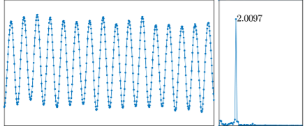
This works great for signals like this (time signal left, dft right with the frequencies of detected modes labeled):

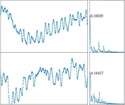
but fails for signals like these (where we see and expect frequencies close to 2; not an order of magnitude smaller!)

Often I expect a certain frequency (e.g f=2.6 in the above signals) and can judge myself the mode is present by the average period between the local maxima. I tried codifying this - computing the average time between local maxima - in MATLAB, but it was pretty unreliable:

[~, peak_inds] = findpeaks(weight);
cycle_periods = diff(peak_inds) * dt;
av_cycle_period = sum(cycle_periods)/length(cycle_periods);
av_freq = 1/av_cycle_period;

My signals are well enough sampled (around 15 to 20 values per observable manky period) to resolve these manky modes visually. I've studied time series and random processes at an undergraduate level, but we never really went too deep into spectral analysis. So:

• How can I reliably compute these highest-frequency modes in my very 'unfourier' signals?

• Why does my current DFT analysis incorrectly deduce very low frequency modes in these manky signals?

• Why would, if multiple present modes have dissimilar frequencies, my naive distance-between-local-maxima-average method fail at extracting the highest frequency?

Answer 1

I think most of your questions can be solved by subtracting then mean from the signal. Namely the all sinusoidal waves, with a nonzero frequency, have a mean of zero. So when the mean of a signal is not close to zero, then it will show up at 0 Hz (you can look at this as $\cos(0\,t)=1$).

After a closer look and some testing by myself it does seem that only removing the mean would not fix your problem. Your signal seems to be contaminated by white noise, which has been integrated probably twice (so low frequencies are much more present than high frequencies). You could try to subtract a higher order polynomial fit, so linear or even quadratic. These fits can easily be obtained using some linear algebra, for example for a quadratic fit:

X = [ones(N, 1), t', t'.^2];
b = (X' * X) \ X' * y';
z = y - (X * b)';

Or you could also look at the biggest peaks above $f^{-2}$, with $f$ the frequency vector. However if you have a signal with normal white noise you should probably just stick with removing the mean, since my proposed methods try to make use of the fact that the present noise is white noise which has been integrated twice.

Answer 2

The reason you see that low-frequency peak is simply because that low frequency component is present in your signal!

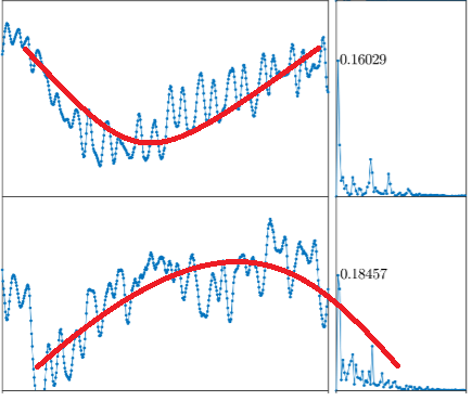
This is very apparent in your time-domain signal as it is biased by (almost) half-period of a very low-frequency sinusoidal.

            

At the same time, the desired component can be distinguished easily in all of your curves as the second peak close to $2$Hz.

if you are not interested in those low-frequencies, you have two choices:

• Ignore the peak in your code if it is in the undesired frequency range (and only accept a frequency if it is in the desired range)
• Apply a high-pass filter to just block the unwanted frequencies and then you can find the highest peak no matter where it is located.