If you're using just straight 2D convolution, you will get the full output. What I think you want is conv2(A, B, 'same').
To better understand this, 1D convolution between two sequences with length N & M results in a final sequence of length = N + M - 1. So without any truncation your conv2 result will no longer be of size 160x160, but (160+M-1)x(160+M-1).
If you're using Matlab, see 'help conv2', 'help filter2', 'help imfilter' (if you have the image processing toolbox installed). imfilter defaults to 'same'.
I'll add a little more discussion regarding filter sizes when they contain exponential functions.
Given in reality were sampling a function that extends to infinity in all directions, albeit the values become insignificant at some point, the function does extend that far. The implementation you're referencing fixes the limits to 3 standard deviations, because that's good enough for them. I saw another implementation that used 8. If you're scale, or sigma, is very large, you run the possibility of the filter turning out to be larger than the image you'll be filtering against. What do you do then? Because like I stated earlier, straight convolution produces a sequence that is N + M - 1.
You need to grab only the central part of that result. The central part would also be of the same size as the image your filtering. That's what the 'same' flag does.
One other point I'd like to make is that there's nothing stopping you from just creating a filter that is the same size as your image. Instead of using sigma as the size controller, just specify the dimension of the filter. Given convolution is often times done in the frequency domain, you're going to be zero padding and taking a larger FFT anyway. Look for references on fast convolution using the FFT.
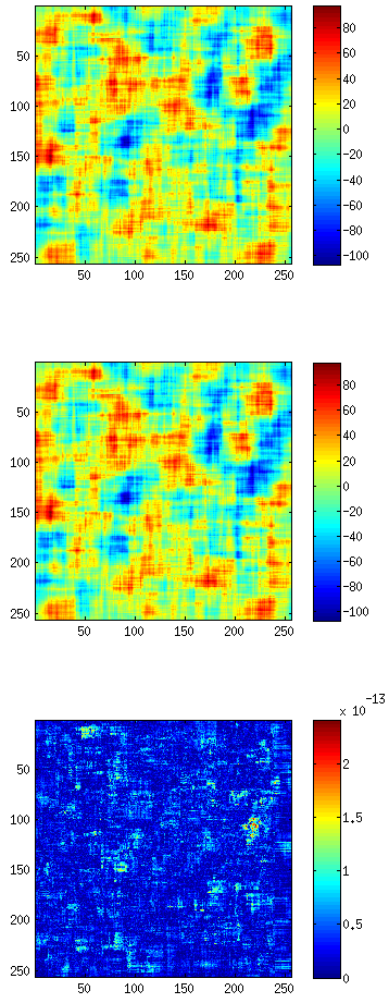
Let's say you're image size is 256x256 and you're filter is 32x32. Here's a simple example without using power of 2 FFT's.
N = 256;
M = 32;
K = N + M - 1; % Length of full convolution

x = randn(N, N);
y = ones(M, M);

% Spatial domain convolution (slow)
r = conv2(x, y, 'same');

% Spatial frequency domain convolution (fast)
z = ifft2(fft2(x, K, K).*fft2(y, K, K));
idx = round((K-N)/2+1):round((K+N)/2); % Indices of the central portion
z = z(idx, idx); % Obtaining the central part of the result

subplot(311), imagesc(r), axis('square'), colorbar
subplot(312), imagesc(z), axis('square'), colorbar
subplot(313), imagesc(abs(r-z)), axis('square'), colorbar


