As the title already says, I would like to know how to calculate the Gain and Phase of a given fixed-point filter at a given frequency.
What I've achieved so far:
Let's say for example that I have a filter with the following difference equation, which corresponds to a Direct Form I biquad structure:
$$
y[k] = b_0 \cdot x[k] + b_1 \cdot x[k-1] + b_2 \cdot x[k-2] + a_1 \cdot y[k-1] + a_2 \cdot y[k-2]
$$
From this difference equation, I can set up the transfer function in the z-Domain, which is:
$$
H(z) = \frac{b_1 \cdot z^2 + b_2 \cdot z + b_3}{z^2 - a_1 \cdot z - a_2}
$$
To turn this back into frequency-domain, I will simply substitute $z$ with $e^{2 \cdot \pi \cdot \frac{f}{f_s}}$, which will give me $H(f)$.
Finally, I can calculate my filter gain by evaluating my function $H(f)$ at the frequency $f$ of interest (assuming the sampling frequency $f_s$ and all coefficients $a_x,b_x$ are known).
The filter gain $G(f)$ is then: $$ G(f) = \sqrt{Re(H(f))^2 + Im(H(f))^2} $$ And the phase $\varphi(f)$ of the filter is: $$ \varphi(f) = atan2(Im(H(f)), Re(H(f))) $$
If multiple stages are cascaded together, then $$ G_{tot} = G_1(f) \cdot G_2(f) \cdot ... $$ and $$ \varphi_{tot} = \varphi_1(f) + \varphi_2(f) + ... $$
Where I currently get stuck:
The above equations have all well worked for double-precision filters.
Now, I would like to do the same calculation for a fixed-point (e.g. 1.15) filter that has fixed-point coefficients, a fixed-point input, a fixed-point output and of course also fixed-point multipliers and adders.
What I don't know is how to deal with these constraints during the calculation.
Do I have to truncate the $e^{2 \cdot \pi \cdot \frac{f}{f_s}}$ terms to the specific fixed-point input precision?
Do I have to use the precision formats of my adders and multipliers to calculate the numerators and denumerators in $H(f)$?
How do I treat the division in $H(f)$, the square root in $G(f)$ and the atan2 in $\varphi(f)$?
Do I have to truncate the final value of $H(f)$ to the specific fixed-point output precision? And if yes, what if an overflow happens?
Any clarifying explanation, literature, video etc. is very welcome, since I haven't found anything valuable by googling. However, I am quite a newbie and might have used the wrong terms for my problem explanation.
Thank you so far @Dan Boschen for your help!
Edit: Where does the gain difference come from???
This afternoon, I was playing around with a fixed-point filter design and simulation in matlab.
I currently try to implement an Order 4 Butterworth Lowpass filter on a microcontroller by using the ARM-CMSIS-DSP Library Documentation (Function arm_biquad_cascade_df1_fast_q15).
This function uses the difference equation that I have previously introduced.
What bothers me is, that the settling value of an input step differs from the value that I would expect when looking at the Bode Plot of my filter and I can't explain why.
This is the Bode Plot of my filter:
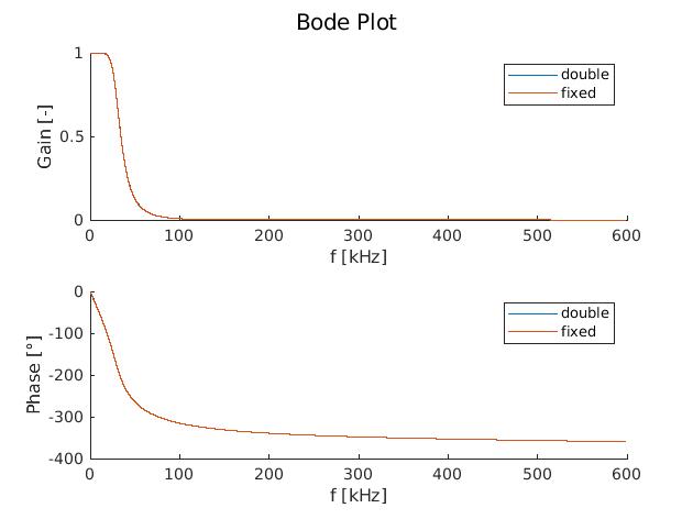
The filter has it's expected properties ($f_s$ = 1.2MHz, $f_c$ = 30kHz) and behaves similar to my "initial" double-precision filter.
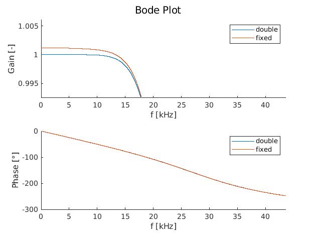
If I zoom in, you can see, that the DC-Gain of my fixed-point filter is a little bit higher than 1 (1.0012), which OK.
If I however apply a 0.5 step to my signal, I get an output that settles to a value that is lower than 0.5 (from the step response settling value, the DC-Gain is 0.9738).
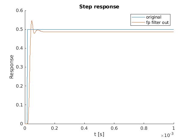
Even if the gain difference is not very big, I still would like to know where it comes from and why.
This is the matlab code that I used to calculate, simulate and plot everything.
clc; clear;

%% Calculate filter coefficients

fs = 1200e3;     %Sampling frequency [Hz]
fc = 30e3;      %Butterworth filter cuttoff frequency [Hz]
n = 4;          %Butterworth filter order

%Get low-pass butterworth filter zeroes and poles
[z, p, g] = butter(n, 2 * fc / fs, 'low');

%Convert zeroes and poles into SOS coefficients
sos_matrix = zp2sos(z, p, g, 'down', 'two');

nCascadedFilterSections = length(sos_matrix(:,1));

%Get double-precision filter coefficients according to my difference equation
%Note: The a coefficients must be multiplied by -1 because matlab uses a
%different difference equation than the CMSIS-Standard
b0_double =  sos_matrix(:, 1);
b1_double =  sos_matrix(:, 2);
b2_double =  sos_matrix(:, 3);
a1_double = -sos_matrix(:, 5);
a2_double = -sos_matrix(:, 6);


%Calculate the required post shift bit to scale all coefficients to my
%fixed-point range [-1 1)
maxValInSos = max(abs(sos_matrix(abs(sos_matrix) > 1)));

if (isempty(maxValInSos))
    postShift = 0;
else
    postShift = ceil(-log2(1 / maxValInSos));
end


%Get 1.15 signed [-1,1) format fixed-point coefficients by truncating the
%scaled double-precision values. Assign previously defined math properties to each
%variable
b0_fixed = fi(b0_double * 2^-postShift, true, 16, 15, fimath('RoundingMethod', 'Nearest'));
b1_fixed = fi(b1_double * 2^-postShift, true, 16, 15, fimath('RoundingMethod', 'Nearest'));
b2_fixed = fi(b2_double * 2^-postShift, true, 16, 15, fimath('RoundingMethod', 'Nearest'));
a1_fixed = fi(a1_double * 2^-postShift, true, 16, 15, fimath('RoundingMethod', 'Nearest'));
a2_fixed = fi(a2_double * 2^-postShift, true, 16, 15, fimath('RoundingMethod', 'Nearest'));

%% Calculate transfer function

%Anonymous Filter Transfer-Function
H = @(z, b0, b1, b2, a1, a2) ((b0 .* z.^2 + b1 .* z + b2) ./ (z.^2 - a1 .* z - a2));

f = 0 : 1 : fs / 2 - 1; %Frequency vector [Hz]
z = exp(1i * 2 * pi * f ./ fs); %Calculate frequency-corresponding z vector

%Calculate double-precision filter gain [-] and phase [°]
mag_double = 1;
ph_double = 0;

for (section = 1 : nCascadedFilterSections)
    mag_double = mag_double .* abs(H(z, ...
        b0_double(section), ...
        b1_double(section), ...
        b2_double(section), ...
        a1_double(section), ...
        a2_double(section)));

    ph_double = ph_double + rad2deg(unwrap(angle(H(z, ...
        b0_double(section), ...
        b1_double(section), ...
        b2_double(section), ...
        a1_double(section), ...
        a2_double(section)))));
end

%Calculate fixed-point filter gain [] and phase [°]
%Cast fixed-point variable type back to double (the coefficient value stays
%the same!)
%Multiply variables by postShift value (see CMSIS Documentation)
mag_fixed = 1;
ph_fixed = 0;

for (section = 1 : nCascadedFilterSections)
    mag_fixed = mag_fixed .* abs(H(z, ...
        double(b0_fixed(section)) * 2^postShift, ...
        double(b1_fixed(section)) * 2^postShift, ...
        double(b2_fixed(section)) * 2^postShift, ...
        double(a1_fixed(section)) * 2^postShift, ...
        double(a2_fixed(section)) * 2^postShift));

    ph_fixed = ph_fixed + rad2deg(unwrap(angle(H(z, ...
        double(b0_fixed(section)) * 2^postShift, ...
        double(b1_fixed(section)) * 2^postShift, ...
        double(b2_fixed(section)) * 2^postShift, ...
        double(a1_fixed(section)) * 2^postShift, ...
        double(a2_fixed(section)) * 2^postShift))));
end

%Plot
figure(1)
clf(1)
s2 = subplot(2,1,1);
hold on
plot(f * 1e-3, mag_double)
plot(f * 1e-3, mag_fixed)
xlabel('f [kHz]')
ylabel('Gain [-]')
legend('double', 'fixed')
s1 = subplot(2,1,2);
hold on
plot(f * 1e-3, ph_double)
plot(f * 1e-3, ph_fixed)
xlabel('f [kHz]')
ylabel('Phase [°]')
legend('double', 'fixed')
sgtitle('Bode Plot')

linkaxes([s1, s2], "x");
%% Calculate the step response
t = 0: 1 / fs : 1e-3; %Discrete Time vector [s]

stepHight = 0.5; %Height of the step input [-]
step = [zeros(1,20), stepHight * ones(1,length(t) - 20)]; %Step signal

%Define fixed-point math rules according to my arithmetic precisions
%ARM CMSIS-DSP Library:
%https://www.keil.com/pack/doc/CMSIS/DSP/html/group__BiquadCascadeDF1.html#ga4e7dad0ee6949005909fd4fcf1249b79
%Filter function:
%arm_biquad_cascade_df1_fast_q15()
fixedPointFilterProperties = fimath('CastBeforeSum', true, ...
    'OverflowAction', 'Wrap', ...
    'RoundingMethod', 'Floor', ...
    'ProductWordLength', 32, ...
    'ProductFractionLength', 30, ...
    'ProductMode', 'SpecifyPrecision', ...
    'SumWordLength', 32, ...
    'SumFractionLength', 30, ...
    'SumMode', 'SpecifyPrecision');

%Set fixed point filter properties to coefficients for correct arithmetics
%according to CMSIS
b0_fixed = setfimath(b0_fixed, fixedPointFilterProperties);
b1_fixed = setfimath(b1_fixed, fixedPointFilterProperties);
b2_fixed = setfimath(b2_fixed, fixedPointFilterProperties);
a1_fixed = setfimath(a1_fixed, fixedPointFilterProperties);
a2_fixed = setfimath(a2_fixed, fixedPointFilterProperties);

%Set step signal as input
in = fi(step, true, 16, 15, fixedPointFilterProperties);

%Define fixed-point filter output vector
out = fi(zeros(1, length(in)), true, 16, 15, fixedPointFilterProperties);

%Filter as it would be done by the CMSIS Library function
for (section = 1 : nCascadedFilterSections)
    for (i = 1 : length(in))
        if (i == 1)
            b0_prod = in(i)    * b0_fixed(section);
            b1_prod = 0        * b1_fixed(section);
            b2_prod = 0        * b2_fixed(section);
            a1_prod = 0        * a1_fixed(section);
            a2_prod = 0        * a2_fixed(section);
        elseif (i == 2)
            b0_prod = in(i)    * b0_fixed(section);
            b1_prod = in(i-1)  * b1_fixed(section);
            b2_prod = 0        * b2_fixed(section);
            a1_prod = out(i-1) * a1_fixed(section);
            a2_prod = 0        * a2_fixed(section);
        else
            b0_prod = in(i)    * b0_fixed(section);
            b1_prod = in(i-1)  * b1_fixed(section);
            b2_prod = in(i-2)  * b2_fixed(section);
            a1_prod = out(i-1) * a1_fixed(section);
            a2_prod = out(i-2) * a2_fixed(section);
        end
        accum = b0_prod + b1_prod + b2_prod + a1_prod + a2_prod;

        accum = accum * 2^postShift;

        out(i) = fi(accum, true, 16, 15, fimath('OverflowAction', 'Saturate', 'RoundingMethod', 'Floor'));
    end
    in = out;
end

%Plot step response
figure(2)
clf(2)
hold on
plot(t,fi(step, true, 16, 15, fixedPointFilterProperties))
plot(t, double(out))
xlabel('t [s]')
ylabel('Response')
legend('original', 'fp filter out')
title('Step response')

%Display DC-Gain of Bode-Plot and Step-Response settling value
DC_Gain_FP_Tf = mag_fixed(1)
DC_Gain_FP_Step = double(out(end)) / stepHight

